Youla-based control switching

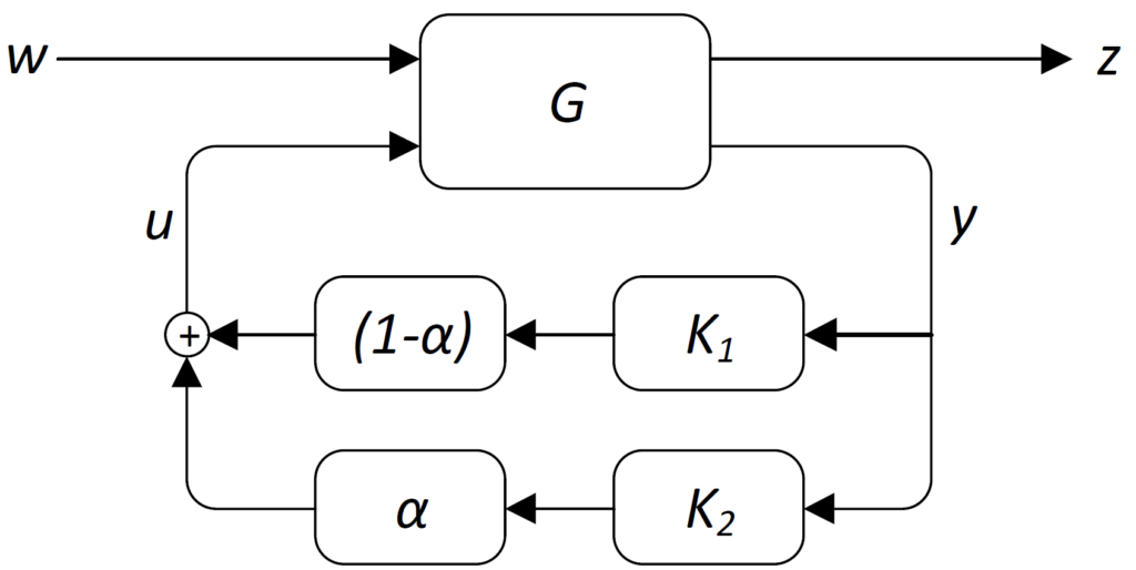
It frequently happens that one would like to implement control-switching schemes to facilitate changing modes, where different controller are subsequently active with the aim to achieve different objectives. Many of such control implementations can be subsumed as shown in the following interconnection.

Here $G$ is the plant to be controlled, while $K=(1-\alpha)K_1+\alpha K_2$ , $\alpha\in[0,1]$ , represents the control switching scheme (i.e. for $\alpha=0$ controller $K_1$ is active, while for $\alpha=1$ controller $K_2$ is active). Here $\alpha$ is a time-varying parameter that in practice is often switched from 0 to 1 in an instantaneous manner. In other more careful implementations, the parameter $\alpha$ is slowly varied for 0 to 1 to facilitate a smoother transitioning between the different controllers.

There are a few issues with this approach:

An instantaneous switch may cause significant disruptions in the closed loop system. The effect is similar to recovering from a nonzero initial condition.
For smoother implementations, where $\alpha$ is varied slowly from 0 to 1, it is unknown if the closed loop system is guaranteed to be stable. This is certainly a problem if either one of the controllers is unstable.

A Youla based solution

To resolve the latter issues, one can proceed according to the approach suggested in [11], [12]. This proceeds as follows.

Let $G$ be a proper LTI system that admits the realization

$G=\left(\begin{array}{cc}G_{11}&G_{12}\\G_{21}& G_{22}\end{array}\right)=\left[\begin{array}{c|cc}A&B_1&B_2\\ \hline C_1&D_{11} &D_{12}\\ C_1&D_{21} &D_{22} \end{array}\right],$

where the pairs $(A,B_2)$ and $(A,C_2)$ are stabilizable and detectable respectively. Then one can compute the coprime factors $G_{22}=NM^{-1}=\tilde{M} \tilde{N}^{-1}$ , which satisfy the Bezout identity

$\left(\begin{array}{cc}\tilde{X}&-\tilde{Y}\\-\tilde{N}&\tilde{M} \end{array}\right) \left(\begin{array}{cc}M&Y\\N&X\end{array}\right)=I,$

where all eight transfer matrices are in $RH_\infty$ .

This can be done using the function fCoprime (details). Given $G$ and the eight transfer matrices that satisfy the Bezout identity, one then can arrive at an entire family of controllers that internally stabilize $G$ .

This parameterization is given by

$K=(Y-MQ)(X-NQ)^{-1}=(\tilde{X}-Q\tilde{N})^{-1} (\tilde{Y}-Q\tilde{M}),$

where $Q$ can be any transfer matrix in $RH_\infty$ . This transfer matrix is the celebrated Youla parameter.

Note that $K$ can also be written as a lower LFT of some fixed transfer matrix $L$ and the Youla parameter $Q$ :

$K=(Y-MQ)(X-NQ)^{-1}= \left(\begin{array}{cc}L_{11}&L_{12}\\L_{21}& L_{22}\end{array}\right)\star Q.$

For a given controller $K$ that internally stabilizes $G$ , even if $K$ is unstable, it is possible to obtain an $L-Q$ interconnection by considering the coprime factors of $K=UV^{-1}=\tilde{V}^{-1}\tilde{U}$ . Then the Youla parameter can be taken to be

$Q=-(\tilde{X}U-\tilde{Y}V)(-\tilde{N}U+\tilde{M}V)^{-1}=$

$=-(\tilde{X}K-\tilde{Y})(-\tilde{N}K+\tilde{M})^{-1}.$

To continue, let us be given two controllers $K_1$ and $K_2$ . Then one can obtain the Youla parameters $Q_1$ and $Q_2$ as sketched above. This leads to the Youla based control-switching scheme depicted in the following figure with:

$Q=(1-\alpha)Q_1+\alpha Q_2,\ \ \ \alpha\in[0,1].$

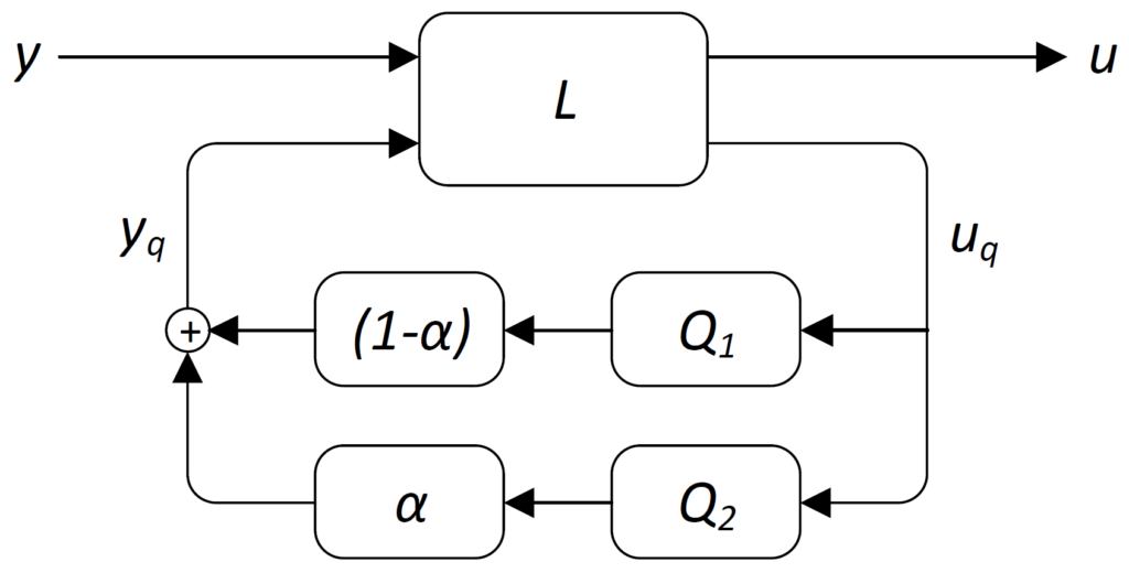
When $\alpha(t)$ is fixed for all $t\in[0,\infty)$ , the Youla parameter $Q=(1-\alpha)Q_1+\alpha Q_2$ is stable, which also implies that the control interconnection of the latter figure is stable. Hence, for any trajectory $\alpha(t)\in[0,1]$ during the switching phase, the resulting controller can be regarded as a linear time varying system. In [11] it is shown that also for this case, the closed-loop system will remain stable.

Note in case $G$ is already stable, i.e., $G\in RH_\infty$ , then the matrices in the Bezout identity may be taken as:

$N=\tilde{N}=G$
$\tilde{X}=M=I$
$X=\tilde{M}=I$
$Y=0$ , $\tilde{Y}=0$

In this case, we obtain $K=-Q(I-GQ)^{-1}=-(I-QG)^{-1}Q$ with the Youla parameter $Q=-U(V-GU)^{-1}=-K(I-GK)^{-1}$ .

Implementation

The function $[L,Q]=fYoulaSwitch(G_{22},K_1,K_2,\cdots,K_N)$ implements the described procedure. Here:

$G_{22}=ss(A,B_2,C_2,D_{22})$ is the part of the plant seen by the controller. This realization must be stabilizable and detectable.
The controllers $K_i=ss(A_i,B_i,C_i,D_i)$ , $i\in{1,2}$ , which both stabilize $G_{22}$ .

As output this yields:

The transfer matrix $L$ with realization $L=ss(A_L,B_L,C_L,D_L)$
The structure $Q$ with the Youla parameters $Q_1,\cdots,Q_N$ .

These can be interconnected as $L\star((1-\alpha)Q_1+\alpha Q_2)$ in accordance with the figure above, or, in case of more than two controllers as $L\star(\alpha_1Q_1+\alpha_2Q_2+\cdots+\alpha_NQ_N)$ with $\Sigma_{i=1}^N\alpha_i=1$ .

Note: The algorithms works for continuous- as well as discrete-time systems.

Demonstrating example

A demonstration of this procedure is found here.