Robust controller synthesis

IQClab also provides the option to perform Robust controller synthesis with general dynamic multipliers. This yields controllers that are robust with respect to the modelled uncertainties.

Note: It is assumed that the user is acquainted with the IQC synthesis literature. The reader is referred to [8], [9] and references therein for further information.

The algorithm considered here is identical to the one presented in [8] , which considers the problem of nominal controller synthesis with unstable weights that have no poles on the imaginary axis [8], [9]. This problem turns out to be very useful in a $\mu$ -like synthesis algorithm for the systematic design of robust controllers with a general linear fractional dependence on the uncertainties. Such algorithms all rely on a suitable factorization of the involved multipliers, which frequently causes numerical ill-conditioning in computations. The present algorithm avoids any such factorizations. If compared to the existing approaches, this leads to a drastically simplified synthesis algorithm for the systematic design of robust controllers based on general dynamic IQC-multipliers.

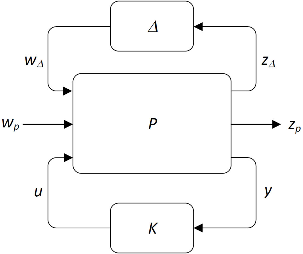
We consider the system interconnection shown in the following figure.

Here:

$P$ is the generalized plant (i.e., it is assumed that the disturbance and performance weights are already incorporated in the plant)
$\Delta$ is the uncertainty block, which is assumed to have a block diagonal structure $\Delta=\mathrm{diag}(\Delta_1,\ldots,\Delta_N)$ . The properties of the individual blocks should be compatible with those from the class iqcdelta (see details here)
$K$ is the to-be-designed robust controller
the in- and output channels are given by
- $w_\mathrm{p}\rightarrow z_\mathrm{p}$ is the performance channel
- $w_\Delta\rightarrow z_\Delta$ is the uncertainty channel
- $u\rightarrow y$ is the control channel

Some characteristics of the algorithm are:

The algorithms performs a synthesis with the aim to obtain a robust controller, $u=Ky$ , which, for all $\Delta\in\mathbf{\Delta}$ , stabilizes the plant $\Delta\star P$ and renders the induced $L_2$ -gain on the performance channel $w_\mathrm{p}\rightarrow z_\mathrm{p}$ less than $\gamma>0$ .
The $\Delta$ -block is compatible with the class iqcdelta (see details here)
The algorithms imposes the following induced $L_2$ norm constraint on the performance channel $w_\mathrm{p}\rightarrow z_\mathrm{p}$ :
$\int_0^{\infty}\left(\begin{array}{c}z_\mathrm{p}(t)\\w_\mathrm{p}(t)\end{array}\right)^T\left(\begin{array}{cc}\frac{1}{\gamma}I&0\\0&-\gamma I\end{array}\right)\left(\begin{array}{c}z_\mathrm{p}(t)\\w_\mathrm{p}(t)\end{array}\right)dt\geq0\ \ \forall t\geq0.$
Here $\gamma$ is the to-be-minimized induced $L_2$ -gain.
The algorithm relies on an iteration between performing nominal (weighted) controller syntheses and IQC robustness analyses. This is similar to the $\mu$ -synthesis approach. The essential different is that the present algorithm allows to consider general dynamic IQC multipliers and does not rely on any factorization of the multipliers.

The algorithm proceeds as follows:

Initialization (iteration step )
1. Design a standard $H_\infty$ controller $K_1$ with $\|P_\mathrm{nom}\star K_1\|\leq\gamma_\mathrm{nom}$
2. Construct the closed-loop system $P\star K_1$ and perform an IQC-analysis. This yields the upper-bound $\gamma_1$ with $\gamma_\mathrm{nom}\leq\gamma_1$ and $\|\Delta\star P\star K_1\|\leq\gamma_1$ for all $\Delta\in\mathbf{\Delta}$ .
Iteration (step for )
1. With the multiplier $\Pi$ from the IQC-analysis for $K_{i-1}$ , design a new controller $K_i$ . Minimization yields the bound $\gamma_\mathrm{rob}^i$ with $\gamma_1\geq\cdots\geq\gamma_\mathrm{rob}^i\geq\gamma_\mathrm{nom}$ and $\|\Delta\star P\star K_i\|\leq\gamma_\mathrm{rob}^i$ for all $\Delta\in\mathbf{\Delta}$ .
2. Build the closed-loop system $P\star K_i$ and perform an IQC-analysis. This yields the bound $\gamma_i$ with $\gamma_1\geq\gamma_2\geq\cdots\geq\gamma_{i-1}\geq\gamma_\mathrm{rob}^i\geq\gamma_i\geq\gamma_\mathrm{nom}$ and $\|\Delta\star P\star K_i\|\leq\gamma_i$ for all $\Delta\in\mathbf{\Delta}$ .
3. Terminate if $|\gamma_{i-1}-\gamma_i|$ is small.

The iteration yields the controllers $K_1, K_2,\ldots, K_{i-1},K_i$ and worst-case induced $L_2$ -gains $\gamma_1\geq\gamma_2\geq\cdots\geq\gamma_{i-1}\geq\gamma_i\geq\gamma_\mathrm{nom}$ , which guarantee $\Delta\star P\star K_i$ to be stable and which render $\| \Delta\star P\star K_i \|<\gamma_i$ for all $\Delta\in\mathbf{\Delta}$ .

Usage:

$[K,\gamma]=fRobsyn(P,\Delta,n_{out},n_{in})$
$[K,\gamma]=fRobsyn(P,\Delta,n_{out},n_{in},options)$

If feasible, the algorithms returns for each iteration:

The stabilizing controllers $K_i=ss(A_{K,i},B_{K,i},C_{K,i},D_{K,i})$ .
The (guaranteed) induced $L_2$ -gain, $\gamma_i>0$ on the performance channel $w_\mathrm{p}\rightarrow z_\mathrm{p}$ of the closed-loop system $\Delta\star P\star K_i$ .

The inputs should be provided as follows:

The LTI plant is assumed to admit the following state space description
$\left(\!\!\!\begin{array}{c}z_\Delta\\z_\mathrm{p}\\y\end{array}\!\!\!\right)\!=\!\left[\!\!\begin{array}{c|ccc}A&B_\Delta&B_\mathrm{p}&B_u\\ \hline C_\Delta&D_{\Delta\Delta}&D_{\Delta\mathrm{p}}&D_{\Delta u}\\C_\mathrm{p}&D_{\mathrm{p}\Delta}&D_\mathrm{pp}&D_{\mathrm{p}u}\\C_y&D_{y\Delta}&D_{y\mathrm{p}}&D_{yu}\end{array}\!\!\right]\!\!\!\left(\!\!\begin{array}{c}w_\Delta\\w_\mathrm{p}\\u\end{array}\!\!\!\right),$
where
- $w_\Delta(\cdot)\in\mathbb{R}^{n_{w_\Delta}$ and $w_\mathrm{p}(\cdot)\in\mathbb{R}^{n_{w_\mathrm{p}}$ are the uncertainty and disturbance inputs
- $z_\Delta(\cdot)\in\mathbb{R}^{n_{z_\Delta}$ and $z_\mathrm{p}(\cdot)\in\mathbb{R}^{n_{z_\mathrm{p}}$ are the uncertainty and performance outputs
- $u(\cdot)\in\mathbb{R}^{n_u}$ is the control input
- $y(\cdot)\in\mathbb{R}^{n_y}$ is the measurement output
- $(A,B_u)$ is stabilizable and $(A,C_y)$ is detectable
The uncertainty block $\Delta=\{\Delta_1,\ldots,\Delta_N\}$ is an iqcdelta object, to which IQC-multipliers have been assigned with iqcassign (see details here).
The plant input and output dimension data and must be specified as follows:
- $n_\mathrm{in}=[n_{w_\Delta};n_{w_\mathrm{p}};n_{u}]$
- $n_\mathrm{out}=[n_{z_\Delta};n_{z_\mathrm{p}};n_{y}]$
The last input, options, is a structure with various options as summarized in the following table.

Options	Description
options.maxiter	This option defines the maximum number of iterations (default = 10).
options.subopt	If chosen larger than 1, the algorithm computes a suboptimal solution $options.subopt\cdot\gamma$ , while minimizing the norms on the LMI variables $\\|X\\|<\gamma$ , $\\|Y\\|<\gamma$ . The default value is 1.05.
options.condnr	If chosen larger than 1, the algorithm computes a suboptimal solution $options.condnr\cdot\gamma$ , while improving the conditioning number of the coupling condition $\left(\begin{array}{cc}Y_{22}&\gamma I\\ \gamma I&X_ {22} \end{array}\right)\succ0$ by maximizing $\gamma$ . The default value is 1.
options.constants	options.constants= $[c_1,c_2,c_3]$ is a vector of (small) nonnegative constants, which perturb the LMIs as $LMI_i\prec-c_i$ , $i\in\{1,2,3\}$ . The constants are associated with the following LMI constraints – $c_1$ perturbs the coupling condition as $\left(\!\!\begin{array}{ccc}Y_{11}+X_{11}&Y_{12}&-X_{12}\\Y_{12}^T&Y_{22}&I\\-X_{12}^T&I&X_{22}\end{array} \!\!\right)\!\succ\!c_1I$ – $c_2$ perturbs the primal solvability condition as $LMI_\mathrm{primal}\prec-c_2I$ – $c_3$ perturbs the dual solvability condition as $LMI_\mathrm{dual}\succ c_3I$ The default value is $1e-9[1,1,1]$ .*
options.gmax	This option specifies the maximum induced $L_2$ -gain bound on the performance channel $w_\mathrm{p}\rightarrow z_\mathrm{p}$ . The default value is 1000.
options.Pi11pos	To improve the conditioning of the IQC-multiplier sub-block $\Pi_{11}$ , it is possible to include the positivity constraint $\Pi_{11}(i\omega)\succ Pi11pos\cdot I\ \ \forall\omega\in\mathbb{R}\cup\{\infty\}.$ To do so, one can specify ‘ Pi11pos’ (default = 0). Note: $\Pi_{11}$ is always positive (semi) definite on the imaginary axis. The reason to include this constraint is to enforce its strictness by means of the non-negative constant ‘Pi11pos’. This option improves the conditioning of the synthesis algorithm.
options.Parser	The option options.Parser specifies which parser is used: – options.Parser=’LMIlab’ – options.Parser=’Yalmip’ The default options is ‘LMIlab’.
options.Solver	The option options.Solver specifies which solver is used when considering Yalmip as parser. See https://yalmip.github.io/ for further info. The default solver is ‘mincx’.
options.FeasbRad	This option allows setting the feasibility radius of the optimization problem (see MATLAB → help → mincx for further details). The default value is 1e9.
options.Terminate	This option can be used to change the LMI solver options (see MATLAB → help → mincx for further details). The default value is 0.
options.RelAcc	This option can be used to change the LMI solver options (see MATLAB → help → mincx for further details). The default value is 1e-4.