Parametric sensitivity analysis

The file Demo_015.m is found in IQClab’s folder demos. In this demo we demonstrate the parametric sensitivity analysis tools presented here.

Let us consider a 3-axis satellite control stabilization problem. The spacecraft attitude is controlled by means of 4 reaction wheels (RWLs) and the closed-loop controlled system interconnection is affected by several parametric uncertainties, namely, the spacecraft inertia (6), the RWL scale factor (4) and misalignments (8), together adding up to 18 uncertainties in total.

The (linearized) plant models of the spacecraft and the RWLs are given by $G=(J_{sc}s^2)^{-1}$ and $G_{rwl}=(J_{rwl}s)^{-1}$ . Here $J_{sc,ij}=J_{ij}(1+w_{ij}\delta_{ij})$ with $\delta_{ij}\in[-1,1]$ ,

$J=\left(\begin{array}{ccc}94.76&0.5929&1.416\\0.5929&125.2&-1.283\\ 1.416&-1.283&65.95\end{array}\right)$

and

$w=\left(\begin{array}{ccc} 0.05&0.5&0.01\\0.5&0.1&0.01\\0.01&0.01&0.5\end{array}\right),$

while $J_{rwl}=0.00106$ .

The (diagonal) attitude controller $K=diag(K_{11},K_{22},K_{33})$ is defined by

$K_{ii}=\frac{0.91(s+0.23)(s^2+0.09s+0.004)}{(s+5.27\cdot10^{-6})(s+1.96)(s^2+1.19s+0.97)}\cdot J_{ii}$

and the RWLs are controlled by means of a PI-controller $K_{rwl}=k_p+k_i/s$ with $k_p=J_{rwl}\omega^2$ , $k_i=2J_{rwl}\alpha\omega^3$ , $\alpha=0.062$ , $\omega=2\pi/T$ , and $T=11.2$ .

This yields the nominal closed-loop RWL model

$H_{rwl}=\frac{0.315(s+0.069)}{(s+0.104)(s+0.211)}.$

As mentioned above, the RWLs are subject to scale factor and misalignment uncertainties. The four RWLs are oriented as

$R=\left(\begin{array}{cccc} -0.5&-0.5&-0.5&-0.5\\ 0.707&-0.707&-0.707&0.707\\-0.5&-0.5&0.5&0.5\end{array}\right).$

The misalignment can then be modelled as

$U_j=\mathrm{null}(R_j^T)w_{rwl,ma}\left(\begin{array}{c}\delta_{rwl_j,ma_x}\\\delta_{rwl_j,ma_y}\end{array}\right)$

where $R_j$ is the $j^{th}$ column of $R$ , $w_{rwl,ma}=0.35\pi/180$ is the misalignment angle, and $\delta_{rwl_j,ma_x},\ \delta_{rwl_j,ma_y}\in[-1,1]$ , $j=1,\cdots,4$ , are the RWL misalignment uncertainties.

Also defining the RWL scale-factor uncertainties $\delta_{rwl_j,sf}\in[-1,1]$ , $j=1,\cdots,4$ , and the weight $w_{rwl,sf}=0.05$ allows defining the overall RWL model as

$F_{rwl}=(R+U)P_{rwl}R^+.$

Here $U=(U_1,\cdots,U_4)$ , $R^+$ is the pseudo-inverse of $R$ , and $P_{rwl}=diag(P_{rwl_1},\cdots,P_{rwl_4})$ with $P_{rwl_j}=H_{rwl}(1+w_{rwl,sf}\delta_{rwl_j,sf})$ .

The closed-loop system is then finally obtained by defining the sensitivity function $S=(I_3+KP_{rwl}G_{sc})^{-1}$ , which is the mapping from the attitude reference input to the tracking error output. The latter is weighted with the performance weighting function

$W_s=\frac{(s^2+0.1s+0.0025)}{(2s^2+4\cdot10^{-5}s+2\cdot10^{-10})}.$

We’re now ready to perform the following sensitivity analyses.

Note: It is emphasized that the controller was not highly tuned and just serves this example for illustrative purposes.

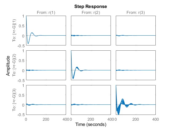
First, the following figure depicts the step response for various samples of the uncertainties. As can be seen, the main uncertainty is observed in the bottom right plot, which presumably is caused by the large uncertainty in $J_{sc,33}$ . This will be confirmed next.

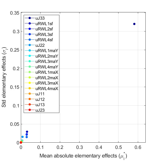
Unit step response from reference input to tracking error output

Let us now perform a sensitivity analysis with Morris method. The following figure depicts the mean (of the absolute value) and standard deviation of the computed elementary effect of each uncertain parameter. As can be seen, there is one main driving uncertain $\delta_{sc,33}$ (i.e., $uJ33$ ) that affects the performance the most. In addition, there are five parameters (i.e., all four RWL scale factors and $\delta_{sc,22}$ ) that have a smaller by observable effect, while the remaining ones have almost no effect.

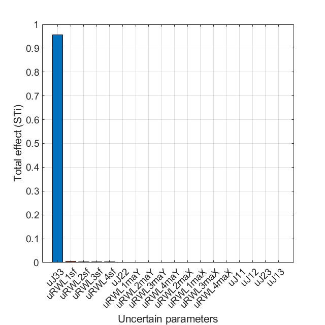
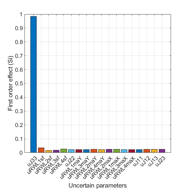
Sensitivity analysis using Morris method

Next to the previous analysis, the following two figures respectively depict the computed total and first order effects obtained by variance-based approach. These confirm the previous conclusions

Sensitivity analysis using the variance based approach (total effect)

Sensitivity analysis using the variance based approach (first order effects)

Finally, for validation purposes, we compute the worst-case gains for:

the nominal system: 0.76
the uncertain system that is affected by the “insensitive” parameters: 0.78
the uncertain system that is affected by the 6 driving uncertainties: 1.52
the uncertain system that is affected by all uncertainties: 1.56

From this we conclude that indeed the worst-case gain for the six driving uncertainties is close to the worst-case gain that was computed for the full uncertain system. On the other hand. the worst-case gain obtained for the system that is only affected by the “insensitive” parameters is close to the one computed for the nominal system.

This all illustrates how the sensitivity analysis can be used to identify driving uncertainties and potentially reduce the computational effort in worst-case analyses for much larger uncertain systems by performing the analysis for a subset of driving uncertainties as identified by the sensitivity analysis.