Nominal and robust controller synthesis for an active suspension system

The file Demo_007.m is found in IQClab’s folder demos; it performs a nominal control design with the functions hinfsyn (for MATLAB) and fHinfsyn (from IQClab). In addition, the demo demonstrates the capability to robustify controllers using the functions musyn (from MATLAB) and again fHinfsyn (from IQClab).

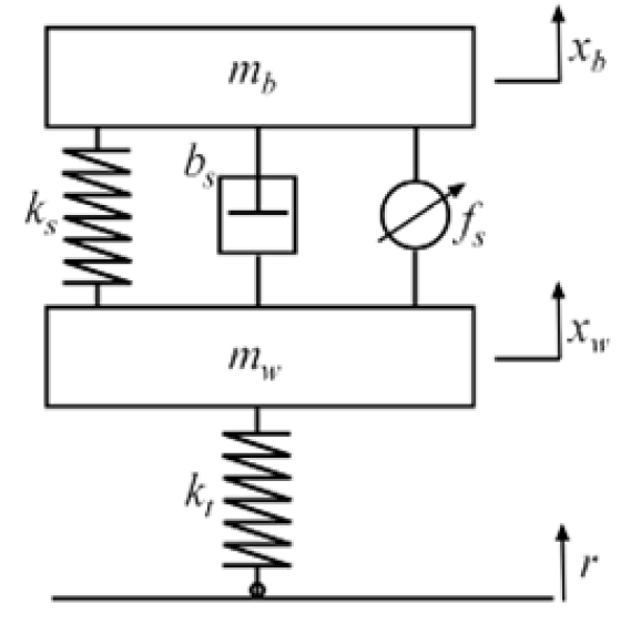
The example is a MATLAB demo: The control design for an active suspension system as depicted in the following figure.

Here:

$x_b$ is the position of the body
$x_w$ is the position of the wheel
$r$ is the position of the road
$m_b$ and $m_t$ are the masses of the body and tire
$k_s$ and $k_t$ are the spring constants of the body and tire
$b_s$ and $f_s$ are the damping and active damping coefficients

With the notation $(x_1,x_2,x_3,x_4)=(x_b,\dot{x}_b,x_w,\dot{x}_w)$ , the linearized state equations are given by:

$\left(\!\begin{array}{c}\dot{x}_1\\ \dot{x}_2\\ \dot{x}_3\\ \dot{x}_4\end{array}\!\right)\!=\! \left(\!\begin{array}{cccc}0&1&0&0\\-\tfrac{k_s}{m_b}&-\tfrac{b_s}{m_b}& \tfrac{k_s}{m_b} & \tfrac{b_s}{m_b}\\0&0&0&1\\ \tfrac{k_s}{m_t}&\tfrac{b_s}{m_w}&-\tfrac{k_s+k_t}{m_w} & -\tfrac{b_s}{m_w} \end{array}\!\right)\!\left(\!\begin{array}{c}x_1\\x_2\\x_3\\x_4\end{array}\!\right)\!+\!\left(\!\begin{array}{cc}0&0\\ \tfrac{10^3}{m_b}&0\\0&0\\ -\tfrac{10^3}{m_w}&\tfrac{k_t}{m_w}\end{array}\!\right) \! \left( \! \begin{array}{c}f_s\\r\end{array}\!\right)$ $\left(\!\begin{array}{c}x_1\\x_1-x_3\\ \dot{x}_2\end{array}\!\right)\!=\!\left(\!\begin{array}{cccc}1&0&0&0\\1&0&-1&0\\ -\tfrac{k_s}{m_b}&-\tfrac{b_s}{m_b}& \tfrac{k_s}{m_b} & \tfrac{b_s}{m_b}\end{array}\!\right)\!\left(\!\begin{array}{c}x_1\\x_2\\x_3\\x_4\end{array}\!\right)\!+ \!\left(\!\begin{array}{cc}0&0\\0&0\\ \tfrac{10^3}{m_b}&0\end{array}\!\right) \! \left( \! \begin{array}{c}f_s\\r\end{array}\!\right)$

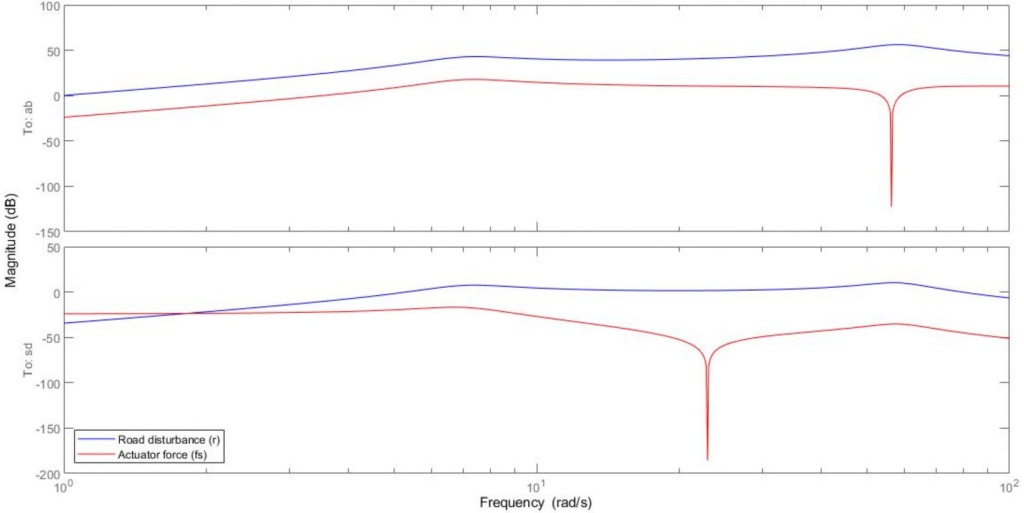
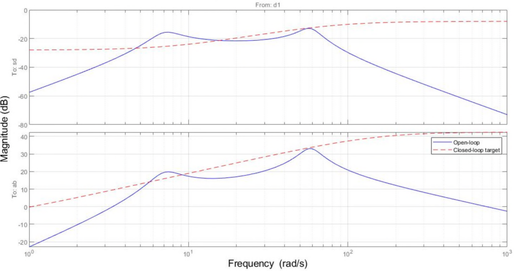
Clearly, road disturbances influence the motion of the car and the suspension. Moreover, passenger comfort is associated with small body accelerations. The allowable suspension travel is constrained by limits on the actuator displacement. The following plot depicts the open-loop gain from road disturbance and actuator force to body acceleration and suspension displacement.

Gain (frequency response) from road disturbance $r$ and actuator force $f_s$ to body acceleration $a_b$ and suspension travel $s_d$ .

Because of the zeros on the imaginary-axis, feedback control cannot improve the response from road disturbance $r$ to body acceleration $a_b$ at the so-called tire-hop frequency, and from $r$ to suspension deflection $s_d$ at the so-called rattle-space frequency. In addition, because $x_w=x_b-s_d$ and $x_w$ roughly follows $r$ at low frequencies (less than 5 rad/s), there is an inherent trade-off between passenger comfort and suspension deflection; any reduction of body travel at low frequency will result in an increase of suspension deflection.

In this example, we consider an uncertain actuator model. This hydraulic actuator used for the active suspension control is connected between the body mass $m_b$ and the wheel assembly mass $m_w$ . The nominal actuator dynamics are represented by the first-order transfer function $\tfrac{1}{(1+60/s)}$ with a maximum displacement of $0.05m$ .

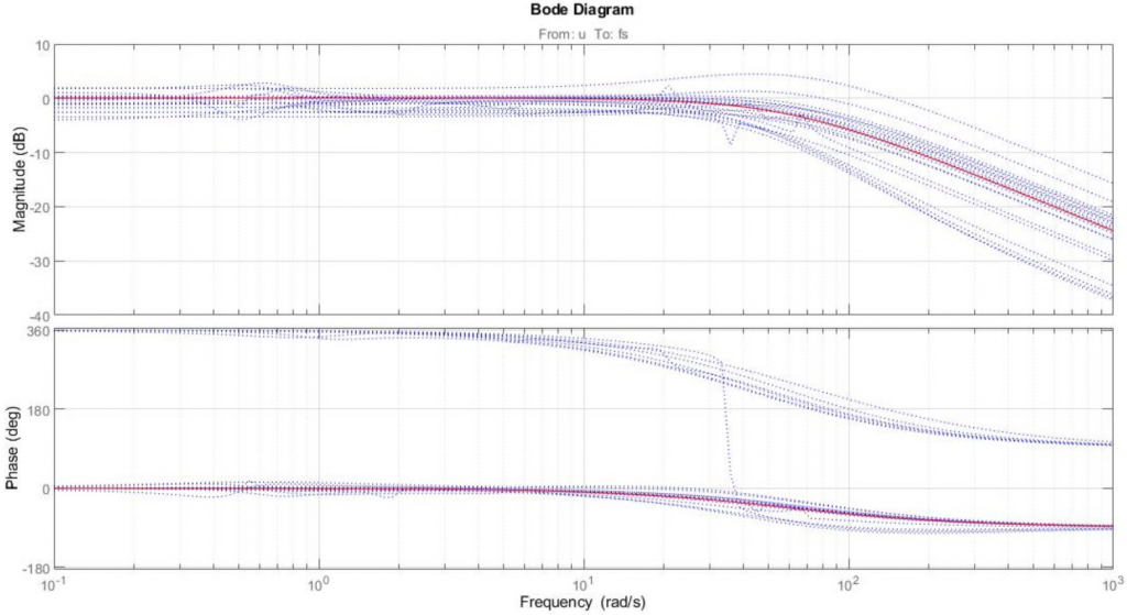
Since the nominal model only approximates the physical actuator dynamics, we can use a family of actuator models to account for modelling errors and variability in the actuator model. This family consists of a nominal model with a frequency-dependent amount of uncertainty. At low frequency, below 3 rad/s, the model can vary up to 40% from its nominal value. Around 3 rad/s, the percentage variation starts to increase. The uncertainty crosses 100% at 15 rad/s and reaches 2000% at approximately 1000 rad/s. The weighting function $W_\mathrm{unc}$ is used to modulate the amount of uncertainty with frequency.

As a result, we obtain $Act$ , which is an uncertain state-space model of the actuator. The following figure depicts the Bode plots of 20 sample values of $Act$ and compare with the nominal value.

Bode diagram of 20 samples of the uncertain actuator model $Act$

The main control objectives are formulated in terms of passenger comfort and road handling, which relate to body acceleration $a_b$ and suspension travel $s_d$ . Other factors that influence the control design include the characteristics of the road disturbance, the quality of the sensor measurements for feedback, and the limits on the available control force. To use the $H_\infty$ -synthesis algorithms, we have to write done the weighted open-loop generalized plant interconnection as shown in the following figure.

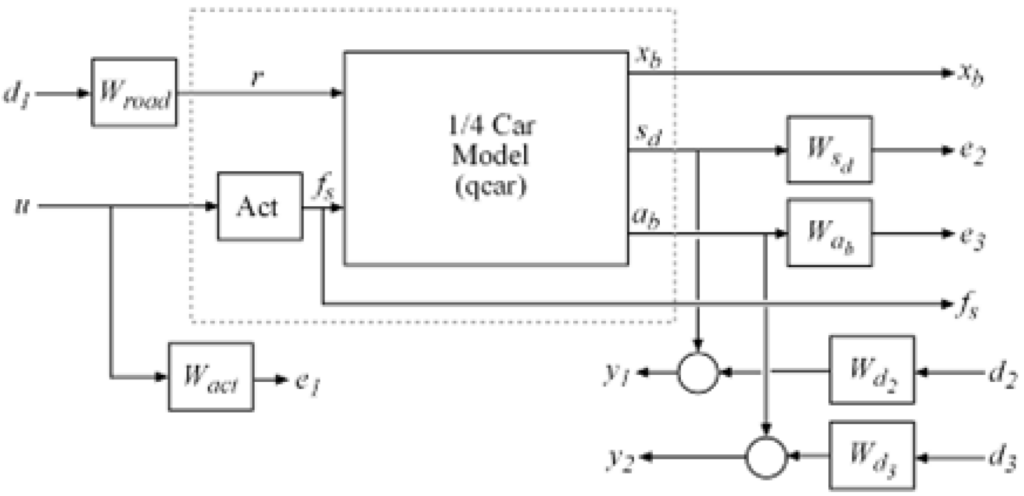
As can be seen, the feedback controller uses measurements $y_1$ , $y_2$ of the suspension travel $s_d$ and body acceleration $a_b$ to compute the control signal $u$ driving the hydraulic actuator. On the other hand, there are three external sources of disturbance:

The road disturbance $r$ , modeled as a normalized signal $d_1$ shaped by a weighting function $W_\mathrm{road}$ . To model broadband road deflections of magnitude seven centimeters, we use the constant weight $W_\mathrm{road}=0.07$ .
Sensor noise on both measurements, modelled as normalized signals $d_2$ and $d_3$ shaped by weighting functions $W_{d_2}$ and $W_{d_3}$ . We use $W_{d_2}=0.01$ and $W_{d_3}=0.5$ to model broadband sensor noise of intensity $0.01$ and $0.5$ , respectively. In a more realistic design, these weights would be frequency dependent to model the noise spectrum of the displacement and acceleration sensors.

The control objectives can be interpreted as a disturbance rejection problem: Minimize the impact of the disturbances $d_1$ , $d_2$ , $d_3$ on a weighted combination of control effort $u$ , suspension travel $s_d$ , and body acceleration $a_b$ . When using the $H_\infty$ -norm to measure “impact”, this amounts to designing a controller that minimizes the $H_\infty$ -norm from disturbance inputs $d_1$ , $d_2$ , $d_3$ to error signals $e_1$ , $e_2$ , $e_3$ .

Let us also create the weighting functions. We use a high-pass filter for $W_\mathrm{act}$ to penalize control at high-frequencies. In addition, we specify the closed-loop performance requirements for the gain from road disturbance $r$ to suspension deflection $s_d$ (handling) and body acceleration $a_b$ (comfort). Because of the actuator uncertainty and control limitations, we only aim for attenuating disturbances below 10 rad/s.

The corresponding performance weights $W_{s_d}$ , $W_{a_b}$ are the inverses of these comfort and handling requirements. To investigate the trade-off between passenger comfort and road handling, we construct three sets of weights $(\beta W_{s_d},1-\beta W_{a_b})$ corresponding to three different trade-offs: comfort ( $\beta=0.01$ ), balanced ( $\beta=0.5$ ), and handling ( $\beta=0.99$ ).

We can now construct the uncertainty model of the generalized plant from above and perform an $H_\infty$ -synthesis using hinfsyn (from MATLAB) and fHinfsyn (from IQClab). The three controllers achieve the following closed-loop $H_\infty$ -norms.

Comfort class	hinfsyn	fHinfsyn
Comfort	0.9405	0.9584
Balanced	0.6727	0.6857
Handling	0.8892	0.9029

Computed $H_\infty$ -norms

Given the controllers $K_1$ and $K_2$ we can now construct the corresponding closed-loop models and compare the gains from road disturbance to $x_b$ , $s_d$ , $a_b$ for the passive and active suspensions. This is shown in the following figure. As can be seen, all three controllers reduce suspension deflection and body acceleration below the rattle-space frequency (23 rad/s). Moreover, both algorithms show very similar performance (which is to be expected).

Frequency responses of the closed-loop system for the controllers obtained by *hinfsyn* (left) and *fHinfysyn* (right).

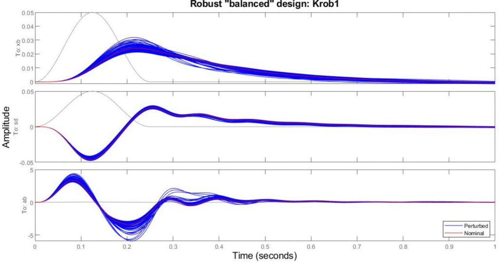
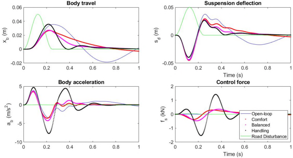
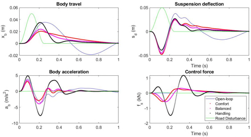
To further evaluate the three designs, let us also perform time-domain simulations using a road disturbance signal $r(t)$ representing a road bump of height 5 cm. The simulation results are shown in the following two figures for the controllers obtained by both algorithms. Here we observe that the body acceleration is the smallest for the controller emphasizing passenger comfort and largest for the controller emphasizing suspension deflection. The “balanced” design achieves a good compromise between body acceleration and suspension deflection. As also can be seen, the results between the different design algorithms are again very similar.

Time-domain response for a road disturbance (*hinfsyn*)

Time-domain response for a road disturbance (*fHinfsyn*)

So far, we have designed $H_\infty$ -controllers that meet the performance objectives for the nominal actuator model. As discussed earlier, this model is only an approximation of the true actuator and it is important to make sure that the controller performance is maintained in the face of model errors and uncertainty.

In fact, by performing a $\mu$ -analysis one can show that the nominal controllers are not capable of guaranteeing robust performance for all possible actuator models in the uncertainty set.

To overcome this problem, we can exploit the $\mu$ -synthesis tools to design a controller that achieves robust performance for the entire family of actuator models. Such robust controller can be synthesized by means of the function musyn using the uncertain model.

On the other hand, it is also possible to exploit fHinfsyn to include the uncertainty channel and impose a weighted small-gain argument to robustify the design.

Both options are presented next for the “balanced” scenario ( $\beta=0.5$ ). The following two figures show the time responses for the robust controllers obtained by hinfsyn and fHinfsyn respectively. As can be seen, both controllers show good time responses for all samples taken from the uncertainty model of the actuator. In fact, the time responses for the controller obtained by fHinfsyn seem to be a little better.

Computing the worst-case gains for both closed-loop system, using wcgain we obtain 0.87 and 1.23 for musyn and fHinfsyn respectively, which implies that the $\mu$ -synthesis algorithm yields slightly better robustness margins.