[latexpage]$H_\infty$-controller synthesis

IQClab offers the possibility to perform $H_\infty$ -syntheses. The algorithm is similar to the (LMI-based) one available in the MATLAB Robust Control Toolbox. However, it offers some additional features that are (currently) not available in the Robust Control Toolbox.

Note: It is assumed that the user is acquainted with the $H_\infty$ -controller synthesis literature and tools. The reader is referred to [3], [4], [5] and references therein for further information.

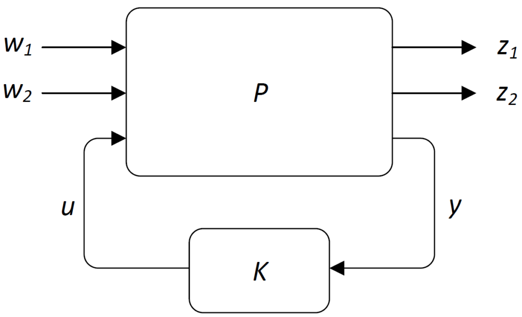
We consider the system interconnection shown in the figure below, where $P$ is the weighted generalized plant (i.e., it is assumed that the disturbance and performance weights are already incorporated in the plant) and where $K$ is the to-be-designed controller. The generalized plant has disturbance inputs $w_1$ and $w_2$ , performance outputs $z_1$ and $z_2$ , control input $u$ , and measurement output $y$ .

Some characteristics of the algorithm are:

The algorithms performs a synthesis with the aim to obtain a controller, $K$ , which stabilizes the plant $P$ and which renders/minimizes the performance specification on the channels $w_1\rightarrow z_1$ and $w_2\rightarrow z_2$ satisfied as detailed next.
The algorithm allows to impose the following norm constraints on the performance channels and respectively:
- A fixed norm-bound, $\alpha$ , on the performance channel $w_1\rightarrow z_1$
  $\int_0^{\infty}\left(\begin{array}{c}z_1(t)\\w_1(t)\end{array}\right)^T\left(\begin{array}{cc}\frac{1}{\alpha}I&0\\0&-\alpha I\end{array}\right)\left(\begin{array}{c}z_1(t)\\w_1(t)\end{array}\right)dt\geq0\ \ \forall t\geq0$
  .
- A to-be-minimized norm-bound. $\gamma$ , on the performance channel $w_2\rightarrow z_2$
  $\int_0^{\infty}\left(\begin{array}{c}z_2(t)\\w_2(t)\end{array}\right)^T\left(\begin{array}{cc}\frac{1}{\gamma}I&0\\0&-\gamma I\end{array}\right)\left(\begin{array}{c}z_2(t)\\w_2(t)\end{array}\right)dt\geq0\ \ \forall t\geq0$
  .
In addition, the algorithm can take initial LMI solutions to invoke warm-starts.

Note: The channel $w_1\rightarrow z_1$ can be included in the synthesis to robustify your control design by imposing the extra norm-constraint (small-gain). Thereby the function allows to include (dynamically weighted) uncertainty channels, which in turn facilitates, for example, $D-K$ iteration type algorithms based on general dynamic multipliers [6].

Usage:

$[K,\gamma]=fHinfsyn(P,n_{out},n_{in})$
$[K,\gamma]=fHinfsyn(P,n_{out},n_{in},options)$
$[K,\gamma,X_e]=fHinfsyn(P,n_{out},n_{in},options)$

If feasible, the algorithms returns:

The stabilizing controller $K=ss(A_K,B_K,C_K,D_K)$
The $H_\infty$ -norm, $\gamma>0$ , on the performance channel $w_2\rightarrow z_2$ of the closed-loop system $P\star K$
The LMI certificate $X_e$

The inputs should be provided as follows:

The LTI plant is assumed to admit the following state space description
$\left(\!\!\!\begin{array}{c}z_1\\z_2\\y\end{array}\!\!\!\right)\!=\!\left[\!\!\begin{array}{c|ccc}A&B_{w_1}&B_{w_2}&B_u\\ \hline C_{z_1}&D_{z_1,w_1}}&D_{z_1,w_2}}&D_{z_1,u}\\C_{z_2}&D_{z_2,w_1}}&D_{z_2,w_2}}&D_{z_2,u}\\C_{y}&D_{y,w_1}}&D_{y,w_2}}&D_{y,u}\end{array}\!\!\right]\!\!\!\left(\!\!\begin{array}{c}w_1\\w_2\\u\end{array}\!\!\!\right),$
where
- $w_1(\cdot)\in\mathbb{R}^{n_{w_1}$ and $w_2(\cdot)\in\mathbb{R}^{n_{w_1}$ are the (generalized) disturbance inputs
- $z_1(\cdot)\in\mathbb{R}^{n_{z_1}$ and $z_2(\cdot)\in\mathbb{R}^{n_{z_1}$ are the performance outputs
- $u(\cdot)\in\mathbb{R}^{n_u}$ is the control input
- $y(\cdot)\in\mathbb{R}^{n_y}$ is the measurement output
- $(A,B_u)$ is stabilizable and $(A,C_y)$ is detectable
In addition, the plant input and output dimension data and should be specified as follows:
- $n_\mathrm{in}=[n_{w_1};n_{w_2};n_u]$
- $n_\mathrm{out}=[n_{z_1};n_{z_2};n_y]$
- Note: In case $n_\mathrm{out}=n_y$ and $n_\mathrm{in}=n_u$ , it is assumed that $n_{w_1}=n_{z_1}=0$ and that the remaining in- and output channels are associated with the second performance channel $n_{w_2}\rightarrow n_{z_2}$ .
The last input, options, is a structure with various options as summarized in the following table.

Options	Description
options.subopt	If chosen larger than 1, the algorithm computes a suboptimal solution $options.subopt\cdot\gamma$ , while minimizing the norms on the LMI variables $\\|X\\|<\gamma$ , $\\|Y\\|<\gamma$ . The default value is 1.01.
options.condnr	If chosen larger than 1, the algorithm computes a suboptimal solution $options.condnr\cdot\gamma$ , while improving the conditioning number of the coupling condition $\left(\begin{array}{cc}Y&\gamma I\\ \gamma I&X\end{array}\right)\succ0$ by maximizing $\gamma$ . The default value is 1.
options.uv	Use different options to reconstruct the controller: – options.uv=1 for $U=X$ and $V=X^{-1}-Y$ – options.uv=2 for $U=Y^{-1}$ and $V=Y$ The default value is 1.
options.eliminate	– options.eleminate=1 solves the controller synthesis problem in one shot (i.e. without eliminating the control variable by projection). – options.eleminate=2 employs the elimination lemma to remove the controller variables form the optimization problem, which allows solving an LMI problem with less optimization variables. The default value is 2.
options.Lyapext	With this option you can specify how the Lyapunov function matrix $X_e$ is constructed. The options are $options.Lyapext\in\{1,2,3,4,5\}$ . The default value is 5.
options.constants	options.constants= $[c_1,c_2,c_3,c_4]$ is a vector of (small) nonnegative constants, which perturb the LMIs as $LMI_i\prec-c_i$ , $i\in\{1,2,3,4\}$ . The constants are associated with the following LMI constraints – $c_1$ , $c_2$ perturb the coupling condition as $\left(\!\!\begin{array}{cc}Y&I\\I&X\end{array} \!\!\right)\!\succ\!\left( \!\!\begin{array}{cc}c_1I&0\\0&c_2I\end{array} \!\!\right)$ – $c_3$ perturbs the primal solvability condition as $LMI_\mathrm{primal}\prec-c_3I$ – $c_4$ perturbs the dual solvability condition as $LMI_\mathrm{dual}\succ c_4I$ The default value is $[0,0,0,0]$ .
options.init	This is a structure with: – options.init. $X_e$ – options.init. $\gamma$ This option can be used to specify an initial condition in the corresponding optimization problem. This option only works for options.eliminate=2 and options.balreal=0. $x_e$ should have twice the size of $A$ , while $\gamma$ is a scalar. The matrices are empty by default.
options.controller	In case options.eliminate=2, you can construct the controller in different fashions by specifying: – options.eliminate=1: This options contructs the controller analytically by means of the function fInvproj (see link for further details) – options.eliminate=2: This option constructs the controller by means of solving an LMI problem. The default value is 1.
options.alpha	This option specifies the maximum $H_\infty$ -norm bound on the performance channel $w_1\rightarrow z_1$ . The default value is 1.
options.gmax	This option specifies the maximum $H_\infty$ -norm bound on the performance channel $w_2\rightarrow z_2$ . The default value is 1000.
options.balreal	This option pre-processes the open-loop weighted generalized plant in the following sense: – options.balreal=0: No balancing is applied – options.balreal=1: A Grammian based IO balancing is applied – options.balreal=2: An $H_\infty$ -Grammian based IO balancing is applied (see the function fHinfbalreal) – options.balreal=3: An norm-balancing is applied by means of the command ssbal. This command computes a diagonal similarity transformation $T$ such that $TB$ and $CT^{-1}$ approximately have equal row and column norms. The default value is 0.
options.Parser	The option options.Parser specifies which parser is used: – options.Parser=’LMIlab’ – options.Parser=’Yalmip’ The default options is ‘LMIlab’.
options.Solver	The option options.Solver specifies which solver is used when considering Yalmip as parser. See https://yalmip.github.io/ for further info. The default solver is ‘mincx’.
options.FeasbRad	This option allows setting the feasibility radius of the optimization problem (see MATLAB → help → mincx for further details). The default value is 1e6.
options.Terminate	This option can be used to change the LMI solver options (see MATLAB → help → mincx for further details). The default value is 0.
options.RelAcc	This option can be used to change the LMI solver options (see MATLAB → help → mincx for further details). The default value is 1e-3.