
The file Demo_001.m is found in IQClab’s folder demos. This demo performs a  – and IQC-robustness analysis for an uncertain plant that is affected by LTI parametric uncertainties. Here it is possible to vary several inputs:
- The uncertainty block:
- One parametric uncertainty that is repeated twice, or
- Two different parametric uncertainties that are repeated once
- Relaxation type:
- DG-scalings
- Convex hull relaxation
- Partial convexity
- Zeroth order Poyla relaxation
- Performance metric:
- Induced
 -gain
-gain  -norm
-norm- Robust stability test
- Induced
The uncertain system is given by  with the open-loop LTI plant
  , where
 ,
,  ,
,  ,
,  ,
,
while:
 for Option 3.1 and Option 3.3,
 for Option 3.2.
On the other hand, the uncertainty block is defined by:
 with
with ![\delta\in[-\alpha,\alpha]](https://usercontent.one/wp/www.iqclab.eu/wp-content/ql-cache/quicklatex.com-49eeea6b9eebbcccb36d25891259fa81_l3.png?media=1702023987 "Rendered by QuickLaTeX.com") , for Option 1.1, or
, for Option 1.1, or with
with ![\delta_1\in[-\alpha_1,\alpha_1]](https://usercontent.one/wp/www.iqclab.eu/wp-content/ql-cache/quicklatex.com-024892574aca1a7ad232bb945e7f6350_l3.png?media=1702023987 "Rendered by QuickLaTeX.com") ,
, ![\delta_2\in[-\alpha_2,\alpha_2]](https://usercontent.one/wp/www.iqclab.eu/wp-content/ql-cache/quicklatex.com-edb661902d1ba00026f1762d02389002_l3.png?media=1702023987 "Rendered by QuickLaTeX.com") for Option 1.2.
for Option 1.2.
The demo file Demo_001.m allows to run an IQC-analysis for various values of ![\alpha\in[0,1]](https://usercontent.one/wp/www.iqclab.eu/wp-content/ql-cache/quicklatex.com-8d1a0bdc10aa5d9a9cd33815a79df449_l3.png?media=1702023987 "Rendered by QuickLaTeX.com") and within the file one can change the inputs mentioned above. For illustration purposes, the following 5 lines of code specify an IQC-analysis for the uncertain plant
and within the file one can change the inputs mentioned above. For illustration purposes, the following 5 lines of code specify an IQC-analysis for the uncertain plant  , for
, for  and the induced -gain as performance metric. In addition, the following parameters are considered:
- Relaxation type: ‘CH’ (Option 2.2)
- Length of the basis function: 2
- Solution check: ‘on’
- Enforce strictness of the LMIs:

% Define uncertain plant
M = ss([-2,-3;1,1],[1,0,1;0,0,0],[1,0;0,0;1,0],[1,-2,0;1,-1,1;0,1,0]);

% Define uncertainty block
de = iqcdelta('de','InputChannel',1:2,'OutputChannel',1:2,'Bounds',[-0.5,0.5]);

% Assign IQC-multiplier to uncertainty block
de = iqcassign(de,'ultis','Length',3,'RelaxationType','CH');

% Define performance block
pe = iqcdelta('pe','ChannelClass','P','InputChannel',3, 'OutputChannel',3,'PerfMetric','L2');

% Perform IQC-analysis
prob = iqcanalysis(M,{de,pe},'SolChk','on','eps',1e-8);
To continue, if running the IQC analysis in Demo_001.m for
 (Option 1.1)
- Convex hull relaxation (Option 2.2)
- Induced -gain performance (Option 3.1)
you obtain as output the worst-case induced -gain for increasing values of computed by the -tools (command: wcgain) and the IQC-tools for different lengths of the basis function. This yields the results shown in the following figure. As can be seen, the IQC-analysis produces worst-case induced -gains (i.e.  -norms in this example), which are consisted with the -analysis. For static multipliers (case:
  , red dashed-line) the
  -level increases faster than the others, at the benefit of a lower computational load. On the other hand, for basis-lengths larger than
  , the results coincide the -analysis up to values of
  . Choosing higher basis-lengths would allow to converge even further.
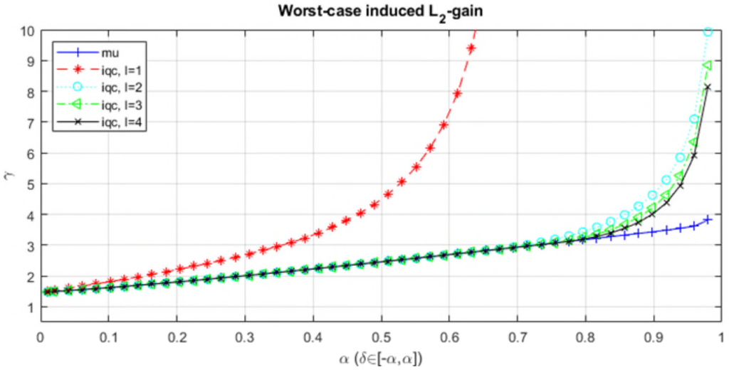 -gain for increasing values of
  and different lengths of the basis function