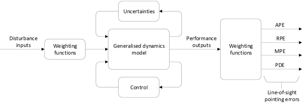
Robust pointing performance tools

IQClab facilitates the robustness analysis and control design for attitude and orbital control systems (AOCS) (i.e. pointing systems) by means of dedicated performance weighting functions.

In other words, IQClab allows defining dedicated pointing matrices, which yield the quality of the pointing as a function of the variability of the system in the presence of the modelled uncertainties. This is illustrated in the following figure.

A main advantage of IQClab is that it facilitates the direct minimization of the $H_2$ -norm, which is not possible with the $\mu$ -tools.

Pioneering work in this direction, especially on the definition of the weighting functions, was performed by Pittelkau (see e.g., [13]). The application of such weights in the $H_\infty$ setting and using the $\mu$ -tools was presented in [14].

The following figure depicts some relevant performance error metrics have been defined by the European Cooperation for Space Standardization (ECSS) in, for example ECSS-E-ST-60-10C.

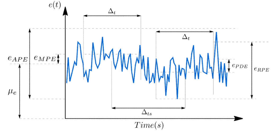
Here the error metrics are defined by:

\[e_\mathrm{APE}=n_p\sigma_\mathrm{APE} +|\mu_e|.\]

The term $n_p$ denotes the confidence level of the requirement (e.g., $n_p =1$ for 68.3%, $n_p = 2$ for 95.5% and $n_p = 3$ for 99.7%). It is emphasized that the standard deviation of the RPE requirement depends on the specified time interval $\Delta_t$ , while the PDE requirement depends on both $\Delta_t$ and the time between intervals $\Delta_{ts}$ . In addition, the standard deviation, denoted by $\sigma$ , of the above metrics can be analysed by means of the PSD of the pointing error signals, which are assumed to be zero-mean stationary random processes.

To exemplify this, let us analyse a generic pointing error $e_\mathrm{metric}$ and let us define the uncertain plant $e=P(\Delta)d$ , which we assume to admit an LFT description, and where $d$ and $e$ denotes the generalized disturbance input and pointing performance error output respectively. The standard deviation of the pointing error signal $e_\mathrm{metric}$ can be evaluated in the frequency domain (for SISO system as

$\sigma_\matrm{metric}(\omega,\Delta_t)=\sqrt{\dfrac{1}{2\pi}\int_0^{\infty}W_\mathrm{metric}(\omega,\Delta_t)G(\omega)d\omega},$

where $G$ is the single-sided PSD of $e$ and $W_\metric$ is the PSD of the pointing error metric, which captures the characteristics of the pointing error metric. Here some of the metrics use time windows, which take the form of sinc-functions in the frequency domain.

Hence, for the linear analysis, we need to rely on rational approximations $\tilde{W}_\mathrm{metric}$ , such that $W_\mathrm{metric}(\omega)\approx| \tilde{W}_\mathrm{metric}(i\omega)|^2$ for $\omega\in[0,\infty]$ . For the metrics above, these are given in the following table.

\tilde{W}_\mathrm{MPE}(i\omega,\Delta_t) =\dfrac{2(i\omega\Delta_t+6)}{(i\omega\Delta_t)^2+6( i \omega\Delta_t)+12}

The function $W=fPEET(type,\Delta_t ,\Delta_{ts})$ generates the latter weighting functions.

The inputs should be specified as follows:

Type of metric
- type=’ape’ for absolute performance error
- type=’mpe’ for mean performance error
- type=’rpe’ for relative performance error
- type=’pde’ for performance drift error
$\Delta_t$ for the time window (required for type=’mpe’, type=’rpe’, and type=’pde’)
$\Delta_{ts}$ for the time interval (required for type=’pde’)

Index	Description
APE	The absolute performance error (APE) is the difference between the target- and the actual pointing direction: $e_\mathrm{APE}=n_p\sigma_\mathrm{APE} +\|\mu_e\|.$
RPE	The relative performance error (RPE) is the difference between the APE at a give time within a time interval $\Delta_t$ , and the mean value of the APE over the same time interval: $e_\mathrm{RPE}=n_p\sigma_\mathrm{RPE} (\Delta_t).$
MPE	The mean performance error (MPE) is the mean value of the APE over a specific time-interval $\Delta_t$ : $e_\mathrm{MPE}=n_p\sigma_\mathrm{MPE} +\|\mu_e\|.$
PDE	The performance drift error (PDE) is the difference between the MPEs taken over two time intervals separated by a specified time $\Delta_{ts}$ within a single observation period: $e_\mathrm{PDE}=n_p\sigma_\mathrm{ PDE } (\Delta_t,\Delta_{ts}).$

Index	Rational approximation
APE	$\tilde{W}_\mathrm{APE}=1$
MPE	$\tilde{W}_\mathrm{MPE}(i\omega,\Delta_t) =\dfrac{2(i\omega\Delta_t+6)}{(i\omega\Delta_t)^2+6( i \omega\Delta_t)+12}$
RPE	$\tilde{W}_\mathrm{RPE} (i\omega,\Delta_t) =\dfrac{i\omega\Delta_t(i\omega\Delta_t+\sqrt{12})}{(i\omega\Delta_t)^2+6(i\omega\Delta_t)+12}$
PDE	$\tilde{W}_\mathrm{PDE} (i\omega,\Delta_t,\Delta_{ts})=\tilde{W}_\mathrm{MPE}(i\omega,\Delta_t)\dfrac{2i\omega\Delta_{ts}(i\omega\Delta_{ts}+6)}{(i\omega\Delta_{ts})^2+6(i\omega\Delta_{ts})+12}$