fMOR – IQClab

The first model order reduction tool is a balanced truncation algorithm that allows performing model order reductions for stable continuous-time LTI systems. This proceeds as follows:

The function $G_\mathrm{red}=$ fMOR $(G,w,T,n,disp)$ performs a model (i.e., state reduction) on the stable MIMO system $G=ss(A,B,C,D)$ .

Here the inputs, if specified, denote:

$G$ is the model
$\omega$ is a frequency vector (covering the design frequency range for plotting (e.g., $\omega=logspace(-3,2,100)$ )
$T=$ ‘name’ is the title of the figure
$n$ is the desired state dimension of the reduced system
$disp=$ ‘off’ turns off the graphical interface

Note: If $n$ is chosen as $0<n<1e-2$ , the system only removes uncontrollable and unobservable states with a tolerance of (i.e., the Hankel singular values with a magnitude of) $n$ .

As output, you obtain the reduced system $G_{red}$ .

Example

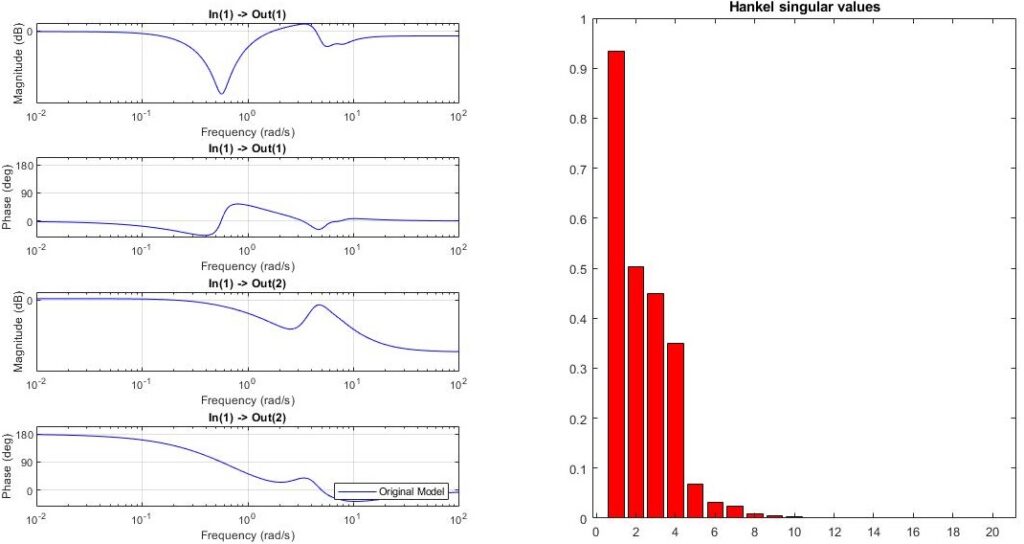
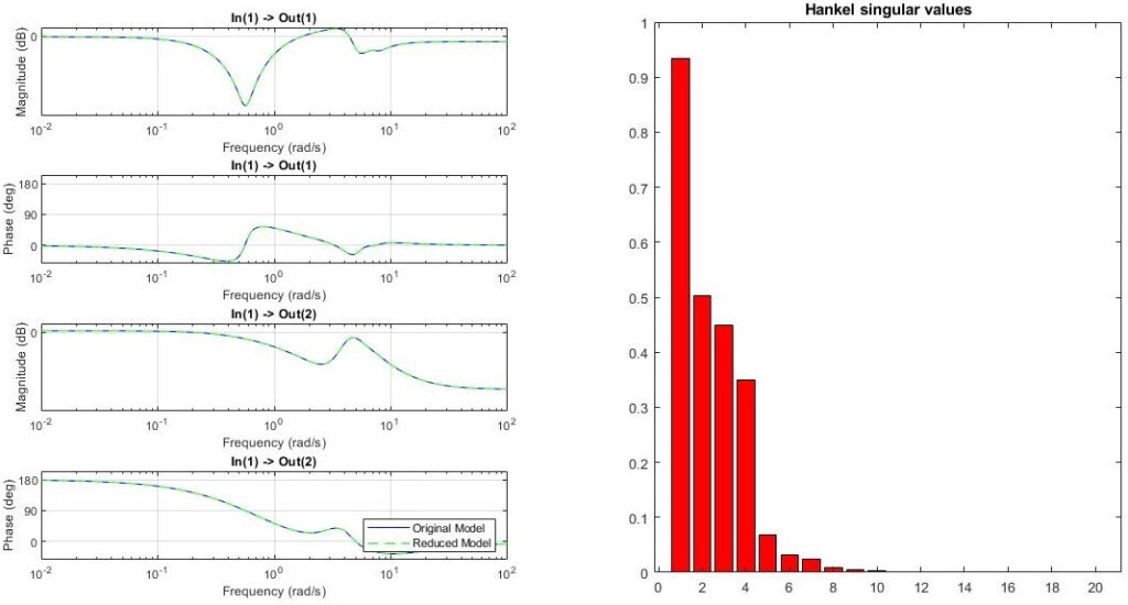
The following code generates a random $2\times 1$ state space model with $20$ states. The function then plots the Bode plots together with the Hankel singular values as shown in the figure. Subsequently, the user is asked to specify the model order, after which the Bode plots of the reduced order model are plotted in the same figure as shown below. This allows to directly assess the quality of the reduced order model (in terms of Bode diagrams).

G = rss(20,2,1);
w = logspace(-2,2,1000);
Gred = fMOR(G,w)