Intro – IQClab

The robust control approach

In many control related applications, it is essential to assess stability and performance characteristics of feedback loops. Control algorithms are typically designed based on mathematical models that capture the behaviour of the considered dynamical system. In reality, however, it is not possible to obtain “perfect” representations of such systems. In other words, there is always a mismatch between a mathematical model and the corresponding reality. This is where the robust control framework comes in; it aims for capturing this “mismatch” by means of so-called uncertainties. Examples are:

Physical parameters are often only known within a certain range;
Dynamical models are typically only representative in the lower frequency range;
Measurement and actuation delays are often not included in a design task;
Nonlinear and/or time-varying behaviour is frequently ignored or overly simplified.

One of the key ingredients of the robust control framework is to consider uncertain dynamical systems that are composed of a nominal system $G$ and a “trouble making component” $\Delta$ representing the uncertainty. This is illustrated in the following figure. Here $G$ is (usually) a known stable linear time invariant (LTI) system, while $\Delta$ is an unknown bounded and causal operator from some given set $\mathbf{\Delta}$ that identifies the structure and nature of the uncertainty.

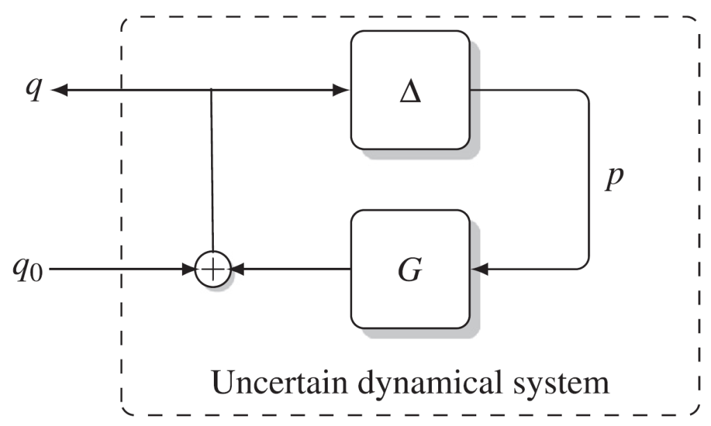
Standard feedback interconnection for robust stability analysis

A fundamental questions here is: How can we systematically verify for all modelled uncertainties $\Delta\in\mathbf{\Delta}$ whether such a system is stable and satisfies a certain performance requirement?

Much research has been carried out in this direction, which has led, for example, to the well-known $\mu$ or structured singular value framework [17]. The literature in this direction is vast. The reader is referred to textbooks such as [18], [19] and references therein.

These results have proven to be extremely powerful in many practical control applications by the virtue of MATLAB’s Robust Control Toolbox!

The IQC-framework

While the $\mu$ -tools offer the possibility to systematically perform robustness analyses and controller syntheses for LTI systems (i.e., both $G$ and $\Delta$ are LTI), there often is a need for considering larger classes of uncertainties. For example, systems might be varying in time, or be subject to nonlinear behaviour:

The dynamics of an airplane vary significantly with the altitude and Mach-number (among other parameters);
A launcher’s mass, inertia, and centre-of-mass significantly change within a very short time-window after lift-off;
Many control systems have a limited actuation capacity, leading to (nonlinear) actuator saturation issues.
Many control systems cover mode transitions, where one control becomes active, while another one is deactivated. This is also a time-varying system.

Here is where the integral quadratic constraint (IQC)-approach can help you. The IQC-framework, which was introduced by [20], offers the advantage to consider a much larger class of uncertainties if compared to the $\mu$ -approach. Among others, one could think of:

Time-invariant and time-varying parametric uncertainties
LTI dynamic uncertainties
Time-delay uncertainties
Passive and norm-bounded nonlinearities
Sector-bounded and slope restricted nonlinearities

The reader is referred to the tutorial paper, [1], for an introduction to the IQC-framework and references therein to the many contributions that have been made in this direction.

Which problems can you consider with IQClab?

In a practical industrial setting, control engineers often confine there efforts to applying more conventional techniques based on, for example:

Single input single output (SISO) PID control, and variations thereof
Bode, Nyquist, Nichols diagrams
Computation of gain, phase, and delay margins
Computation of eigenvalues, singular values
Time-domain (e.g., Monte Carlo) simulations

These techniques have proven to be extremely useful in millions of practical applications and continue to do so. However, control systems tend to become more and more complex, calling for more advanced approaches such as the $\mu$ – and IQC-framework as further motivated in the following examples.

SISO versus MIMO systems
Conventional design and analysis approaches are sometimes limited to single-input single-output (SISO) systems, while many modern control applications comprise multi-input multi-output (MIMO) systems.

Indeed, many dynamical systems consist of multiple control loops that may be highly coupled (i..e., commands in one input channel may yield responses in more than one output channels). Here it is essential to be able to analyse the control stability and performance of the overall system, rather than only considering the individual loops, which might yield results that are too optimistic, not providing guarantees for the overall system.

Here is where the $\mu$ and IQC-approaches offer a great advantage. They are fully capable of addressing control problems in a multivariable setting.

Time-invariant versus time-varying systems
Classical formal analysis approaches do not offer the possibility to address time-varying systems (other than just performing time-domain simulations).

Here is where the IQC-approach offers an effective solution. Within the IQC-framework, it is possible to consider the class of so-called LPV-systems, which admit the form:

$\begin{array}{l}\dot{x}(t)=A(p(t))x(t)+ B(p(t))u(t)\\ y(t)=C(p(t))x(t)+ D(p(t))u(t) \end{array}$

Here $p$ is a time-varying parameter vector, often called the scheduling parameter, which lives in some (convex) set $\mathbf{p}$ , while the constant state-space matrices $A$ , $B$ , $C$ , and $D$ rationally depend on $p$ . There are even generalizations to this.

LPV models are a very effective way to obtain system descriptions that are valid over a large operational domain, which offers the possibility to perform global stability and performance analyses rather that local ones. As an example, you could think of an airplane model with the altitude and Mach number representing the scheduling parameters.

In addition, it is also possible to systematically design (nonlinear) LPV controllers that provide stability and performance guarantees for an entire operational domain (as opposed to designing local controllers based on local linearizations that are interconnected via heuristic gain-scheduling techniques). For more details click here.

Nominal versus uncertain systems
Conventional formal methods, are very limited in assessing whether a system is stable in the presence of uncertainties.

Indeed, the computation of gain- and phase-margins is not a very adequate approach for confirming whether systems are robustly stable and performing with respect to a set of modelled uncertainties. As mentioned above, this is of paramount importance for the certification of complex control systems, which might be subject to various sources of uncertainties.

Again, here is where the $\mu$ – and IQC-tools offer very powerful means to address such problems. The $\mu$ -tools allow to systematically verify the robust stability and performance properties of LTI systems, which may be affected by real/complex parametric and LTI dynamic uncertainties. In addition, the IQC-tools are capable of handling a much richer class of uncertainties such as time-invariant/time-varying uncertainties possibly with bounds on the rate of variation, LTI dynamics, delay, nonlinearities (saturation, dead-zone), among many others.

Linear versus nonlinear systems
Many conventional formal analysis methods, consider linear or linearized system, while neglecting any form of nonlinearity in the analysis.

On the other hand, many control systems include nonlinear effects that should be included in the analysis. Here you could think of actuator saturation, pulse width modulation, or other nonlinear effects.

Here is where the IQC-tools offer various relevant and effective solutions for performing stability and performance analysis in the presence of nonlinearities such as saturation, dead-zone, hysteresis, sector-bounded, slope-restricted, norm-bounded, and passive nonlinearities, which may even be time-varying.

Transitions and mode-switches
Mode switches (i.e. the switching between two controllers) is another gap that cannot be easily analyzed using conventional approaches.

Many control systems comprise different operational modes, which rely on different controllers and which must realize different performance objectives.

Such problems can be modelled as an LPV system comprising a switching parameter, which may vary slowly, or arbitrarily fast. This problem is further explained here.

Hence, the IQC-tools offer the capability to systematically address the analysis of mode-switches between different controllers. Without limitation, this can even be done in the presence of other uncertainties.

Precise assessment of stability and performance margins
In formal classical approaches, stability and performance margins are computed with e.g., Bode, Nyquist, and Nichols plots, to obtain the gain-, phase-, and delay-margins.

However, these approaches may yield stability and performance margins that are too optimistic. Here, the $\mu$ -tools are a good alternative. However, only in case of LTI uncertainties. In the case of time-varying uncertainties, on the other hand, the results would potentially also be optimistic.

Here the IQC-tools offer a great advantage, being capable of effectively including a rich class of uncertainties in the analysis, including time-varying uncertainties.

Including external disturbances
Conventional formal analysis approaches frequently just consider reference tracking to control error performances. However, in many complex control systems it is paramount to understand the controller’s performance in the presence of all contributing factors, such as all the external disturbance sources.

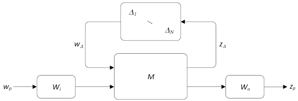
Here the flexible nature of the $\mu$ – and IQC-framework offers the capability to include any external disturbance sources. Subsequently, these can be weighted by means of frequency depended weighting functions that capture the spectral properties of the disturbance source. Such weights may even contain uncertainties.
This is illustrated in the following figure.

Uncertain system interconnection with external disturbance and performance channels.

Including performance channels

Similarly to including external disturbances, it is also possible to add performance channels to the analysis problem. This enables to analyze the impact of external disturbances and uncertainties on the performance of the system.

As before, this proceeds by appending frequency depended weighting functions that capture the performance requirements of the system. In the analysis, this translates into checking if a norm constraint $\|\cdot\|_j$ is smaller than a given constant $\gamma>0$ such that $\|W_\mathrm{o}(\Delta\star M)W_\mathrm{i}\|_j<\gamma$ . The reader is referred to link for an overview of possible metrics.

It is emphasized that this is not limited to checking standard control level performances, such as tracking errors, but also ones that might be related to system level requirements. As an example, we refer to the section robust pointing performance tools, where it is explained how to check various different pointing performance metrics in the context of attitude and orbital control systems (AOCS).

Regional analysis and non-zero initial conditions

Checking performances may also include the computation of invariant (ellipsoidal) sets for the internal state or the output of a system as a result of external disturbances or non-zero initial conditions.

Here it is emphasized that this is fully compatible with considering mixed uncertainties/nonlinearities and (dynamic) IQC-multipliers, offering various benefits, if compared to some of the Lyapunov-based approaches.