
The file Demo_009.m is found in IQClab’s folder demos; it performs a robust controller synthesis with the function fRobsyn. This demo consists of the 2DoF control design for a plant with parametric uncertainty. The plant,  , is a simple oscillator model, which is interconnected as shown in the following figure.

Here is defined by the transfer function
![\[G(s)=\dfrac{1}{k^2s^2+2dks+1},\]](https://usercontent.one/wp/www.iqclab.eu/wp-content/ql-cache/quicklatex.com-e91c35cb0e354dbc94f93e7ab7e204f5_l3.png?media=1702023987 "Rendered by QuickLaTeX.com")
where  is the time-constant and
  the damping factor. Here
  is a fixed constant, while is assumed to be an uncertain parameter
  with
with  and
and ![\delta\in[-1,1]](https://usercontent.one/wp/www.iqclab.eu/wp-content/ql-cache/quicklatex.com-cdc512599dd4884aa5ed731b8f497e43_l3.png?media=1702023987 "Rendered by QuickLaTeX.com") . The bode diagram for various samples of is shown in the following figure.
. The bode diagram for various samples of is shown in the following figure.
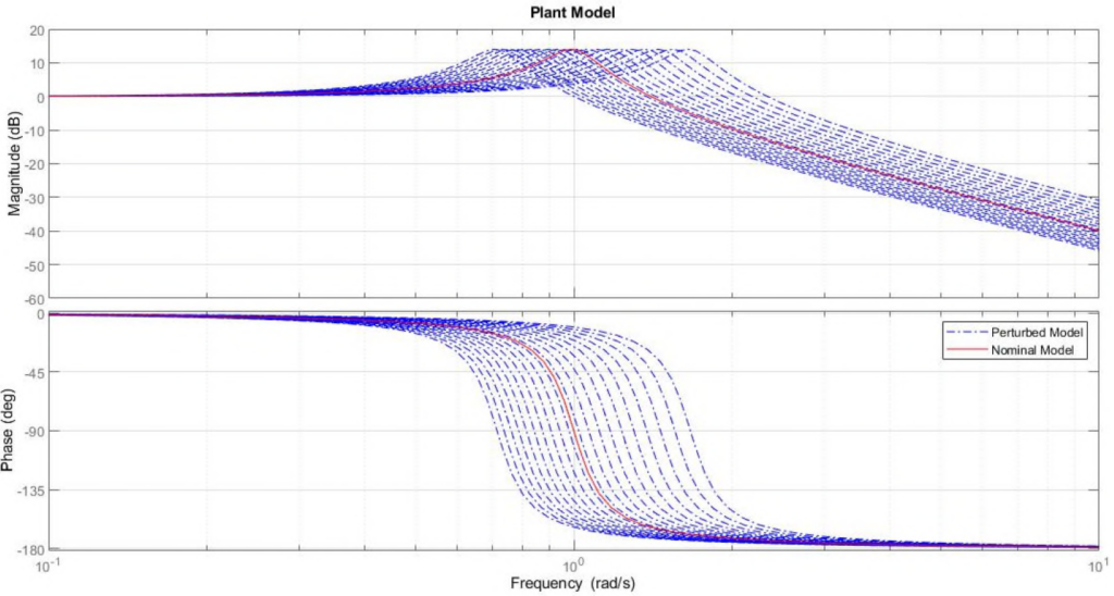
The goal is to design a 2DoF controller,  , which stabilizes the plant for all
 ![\delta\in[−1,1]](https://usercontent.one/wp/www.iqclab.eu/wp-content/ql-cache/quicklatex.com-04ecf6f969366703770037004917aaf8_l3.png?media=1702023987 "Rendered by QuickLaTeX.com") , and which renders the induced
, and which renders the induced  -gain on the weighted performance channels
  satisfied. Here the aim is to enforce good tracking at low frequencies, while penalizing control at high frequencies.
This is accomplished with the performance weights
![\[W_e=\dfrac{(0.5s+0.866)}{(s+0.000866)},\ \ \ W_u=\dfrac{10(s+1)}{(s+100)}.\]](https://usercontent.one/wp/www.iqclab.eu/wp-content/ql-cache/quicklatex.com-020df5f16aaa7118d0f43a660d2248d8_l3.png?media=1702023987 "Rendered by QuickLaTeX.com")
The generalized plant can be constructed as usual (see code in Demo_009.m). Subsequently, you can perform a nominal and robust controller synthesis by means of hinfsyn/fHinfsyn and fRobsyn respectively. The corresponding code is given next.
- Length of the basis function: 3
- Solution check: ‘on’
- Enforce strictness of the LMIs:

% Define the uncertain plant model
k0     = 1;
d      = 0.1;
delta  = ureal('delta',0,'Range',[-1,1],'AutoSimplify','full');
k      = k0*(1+0.4*delta);
G      = tf(1,[k^2,2*d*k,1]);
[H,De] = lftdata(G);
H      = ssbal(H);

% Define the open-loop generalized plant
systemnames  = 'H';
inputvar     = '[p{2};r;u]';
outputvar    = '[H(1:2);r-H(3);u;r;H(3)]';
input_to_H   = '[p(1:2);u]';
cleanupsysic = 'yes';
olic         = sysic;

% Define weights
Wperf = 1/makeweight(1e-3,1,2);
Wcmd  = makeweight(1e-1,10,10);
Wout  = blkdiag(1,1,Wperf,Wcmd,1,1);
wolic = Wout*olic;

% Perform a nominal controller synthesis
[Knom,~,ga_nom] = fHinfsyn(wolic(3:end,3:end),2,1,'method','lmi');

% Define iqc uncertainty block
de = iqcdelta('de','InputChannel',1:2, 'OutputChannel',1:2,'Bounds',[-1,1]);
de = iqcassign(de,'ultis','Length',2);

% perform a robust controller synthesis
options.maxiter   = 5;
options.subopt    = 1.01;
options.constants = 1e-6*ones(1,3);
options.Pi11const = 1e-5;
options.FeasbRad  = 1e5;

[K,ga] = fRobsyn(wolic,de,[2,2,2],[2,1,1],options);
For the nominal controller,  , we obtain an
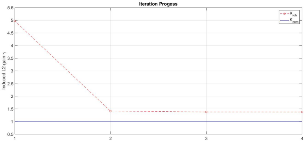
  -norm of approximately 1. However, when performing an IQC-analysis, the worst-case performance is in fact about 10 times larger. The robust controller,
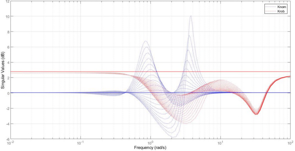
  , on the other hand, guarantees that the worst-case performance is not larger than 1.37, which is much closer to nominal performance level. This is illustrated in the following two figures. As can be seen in the first figure, the function fRobsyn quickly converges after four iterations to a worst-case performance of 1.37. This is confirmed by the second figure, where the sigma plots of the weighted closed loop system are shown for various samples of for both the nominal controller, as well as the robust controller .
 and .
and .To continue, the following figure shows the singular value plots of the sensitivity and control sensitivity function  and
and  respectively, for various samples of versus the inverse weighting functions that were used in the controller synthesis. Again, we conclude that the robust controller, is better capable of guaranteeing performance in the presence of the uncertainty. This is confirmed by the time domain simulation shown in the last figure.
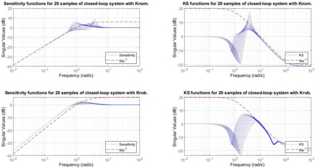
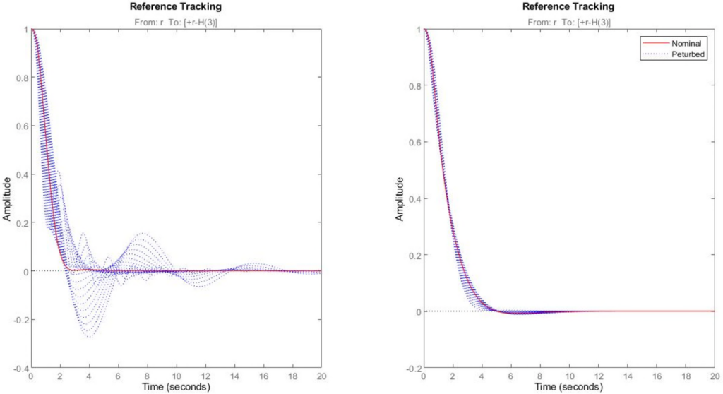 – left: nominal controller, – right: robust controller, .