Regional analysis with LTI parametric uncertainties

The file Demo_013.m is found in IQClab’s folder demos. This demo performs regional analysis following the numerical example reported in [22].

Here the uncertain system is given by $\Delta\star M$ with $\delta\in[-1,1]$ and the open-loop LTI plant

$M=\left(\begin{array}{cc}M_{qp}&M_{qw}\\M_{zp}&M_{zw}\end{array}\right)=\left[\begin{array}{c|cc}A&B_p&B_w\\ \hline C_q&D_{qp}&D_{qw}\\C_z&D_{zp}&D_{zw}\end{array}\right],$

where

$\left(\begin{array}{c|c|c}A&B_p&B_w\\ \hline C_q&D_{qp}&D_{qw}\\ \hline C_z&D_{zp}&D_{zw}\end{array}\right)=$ $\left(\begin{array}{cccc|cc}-0.97&2.34&2.22&3.672&-0.495&0.5843\\-0.21&-0.642&5.042&-0.0998&-0.5587&0.4526\\-2.56&-4.649&-1.071&-9.242&-1.133&0.7273\\-3.64&0.2&9.68&-0.64&0&0\\ \hline 0&-0.1026&0.1026&-0.1625&-0.9099&-0.5017\\ \hline 1.5&-0.11&0&0.93&0&0\\0.1&0&0&0&0&0 \end{array}\right)$ .

The demo file Demo_013.m computes the “smallest” ellipsoid that contains the output trajectory $e$ against disturbances $w$ with $\|w\|\leq1$ . The results are obtained with the following lines of code

% Define uncertain plant
M = ...

% Define uncertainty block
de = iqcdelta('u','InputChannel',1, 'OutputChannel',1,'Bounds',[-1,1]);
de = iqcassign(de,'ultis','Length',4);

% Define performance block
pe = iqcdelta('pe','InputChannel',2,'OutputChannel', 2:3,'ChannelClass','P','PerfMetric','e2z');

% Perform IQC-analysis
prob = iqcinvariance(M,{de,pe},'SolChk','on', 'eps',1e-6);

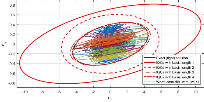
The demo then generates the following figure depicting the ellipsoids obtained for different lengths of the basis function (red lines), the tight ellipsoid (black line) and various worst-case trajectories with $\|w\|\leq1$ and $\delta=-1$ (i.e., the worst case uncertainty).

As can be seen, the IQC-analysis produces non-conservative (tight) ellipsoids for higher lengths of the basis function (dynamic multipliers), while for basis length 1 (static multipliers) we obtain more conservative results, which clearly demonstrates the benefit of considering dynamics in the multipliers.