LPV controller synthesis for a flight control problem

The file Demo_008.m is found in IQClab’s folder demos; it performs an LPV controller synthesis with the function fLPVsyn. The example is taken from [16]. This paper describes the application of the LPV control design algorithm to a parametrically varying flight control problem. The LPV model together with the performance objectives are found in this reference.

The equations of motion are given by:

$\left(\begin{array}{c}\dot{\alpha}\\ \dot{\beta}\\n_z\end{array}\right)=\left(\begin{array}{c}kM\left(\left(a_n\alpha^2+b_n\alpha+c_n\left(2-\dfrac{M}{3}\right)\right)\alpha+d_n u\right)+\beta\\M^2\left(\left(a_m\alpha^2+b_m\alpha-c_m\left(7-\dfrac{8M}{3}\right)\right)\alpha+d_m u\right)\\ M^2\left(\left(a_n\alpha^2+b_n\alpha+c_n\left(2-\dfrac{M}{3}\right)\right)\alpha+d_n u \right) \end{array}\right)$

Here:

$\alpha\in[0,\pi/9]$ is the angle-of-attack (rad)
$u$ is the tail fin deflection (rad)
$\beta$ is the pitch rate (rad/s)
$M\in[2,4]$ is the Mach number
$n_z$ is the normal acceleration per $g$

The remaining constants are given by

$a_n=414.9$
$b_n=-664.9$
$c_n=-208.4$
$d_n=-41.8$
$a_m=49.9$
$b_m=-79.1$
$c_m=3.6$
$d_m=-14.5$
$k=0.001$

The synthesis objective is to track the commanded acceleration manoeuvres $n_{z,r}$ , while satisfying some performance specifications. The control input is the tail fin deflection $u$ , and the measurements are the error in nominal acceleration and the pitch rate:

$y=\left(\begin{array}{c}n_z-n_{z,r}\\ \beta\end{array}\right)$

We choose the reference $n_{z,r}$ for the normal acceleration as the exogenous performance outputs as:

$z_p=W_p\left(\begin{array}{c}n_z-n_{z,r}\\ u\end{array}\right)$

with the performance weight

$W_p=\left(\begin{array}{cc}\dfrac{0.5(s+7)}{(s+3.5\cdot 10^{-6})}&0\\0& \dfrac{4.444\cdot 10^{7}(s+9)}{(s+2\cdot 10^{6})} \end{array}\right)$

in order to enforce disturbance rejection at low frequencies and to penalized control actuation at high frequencies.

To derive the LPV model, we conveniently choose the Mach number, $M$ , and the angle of attack, $\alpha$ , as scheduling variables. Then it is not difficult to formulate an LFT structure of the equations of motion with normalized scheduling block

$\Delta_\mathrm{s}(\delta_M, \delta_\alpha)= \left(\begin{array}{cc}\delta_MI_5&0\\0&\delta_\alpha I_2\end{array}\right)$

where $\delta_M\in[-1,1]$ and $\delta_\alpha\in[-1,1]$ .

The synthesis was run with the following code:

Length of the basis function: 3
Solution check: ‘on’
Enforce strictness of the LMIs: $\epsilon=1e-8$

% Load missile open-loop plant
load missile

% Define uncertainties
del_a = ureal('del_a',0,'Range',[-1,1]);
del_M = ureal('del_M',0,'Range',[-1,1]);
Del_a = pi/18*(1 + del_a);
Del_M = 3 + del_M;
Del_T = blkdiag(Del_a*eye(2),Del_M*eye(5));

% Extract open-loop interconnection for normalized uncertainties
P         = lft(Del_T,ssbal(G));
[olic,De] = lftdata(P);

% Append weighting functions
wp    = ss(tf([0.5,3.5],[1,3.5e-6]));
wu    = ss(20*tf([1/0.9,1],[1e-6,1]));
Wo    = ssbal(blkdiag(eye(7),wp,wu,eye(2)));
wolic = Wo*ssbal(olic);

% Define scheduling block
H{1} = blkdiag(eye(5),zeros(2));
H{2} = blkdiag(zeros(5),eye(2));
La   = polydec(pvec('box',[-1,1;-1,1]))';

iqcdeltaOpt.InputChannel   = 1:7;
iqcdeltaOpt.OutputChannel  = 1:7;
iqcdeltaOpt.Polytope       = La;
iqcdeltaOpt.UncertaintyMap = H;
iqcdeltaOpt.TimeInvTimeVar = 'TV';
iqcdeltaOpt.Structure      = 'FB';

Delta = iqcdelta('Delta',iqcdeltaOpt);

% Define synthesis options
options.RelaxType = 'CH';
options.FeasbRad  = 1e8;
options.constants = [1e-8,1e-7,1e-7,1e-9,1e-8,1e-8];
options.subopt    = 1.1;
options.bounds    = [1e5,1,1e5,1];

% Perform synthesis
[K,ga] = fLPVsyn(wolic,Delta,[7,2,2],[7,1,1],options);

Here

The chosen relaxation type is convex hull (CH),
The feasibility radius is confined to $10^8$ ,
The LMI constraints are perturbed by the constants $10^{-8}[1,10,10,1,1,1]$ ,
A sub-optimal solution is computed, while $\gamma$ is relaxed with 10% and while the norms are minimized with options.bounds= $[10^5,1,10^5,1]$ .

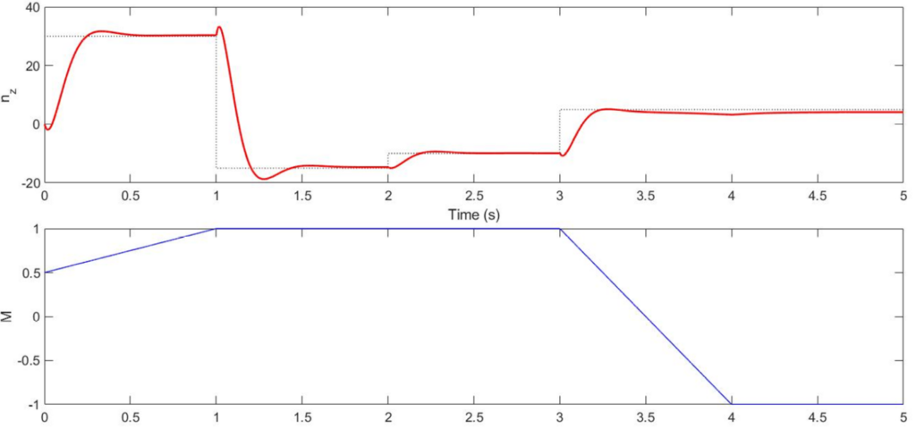
This yields the LTI part of the controller, $K$ , together with the obtained sub-optimal induced $L_2$ -gain, $\gamma=1.74$ . The time-domain simulation results are shown in the following figure.