Anti-windup compensator design for a MIMO control system

The file Demo_010.m is found in IQClab’s folder demos. Here we reproduce the example from [10] with the plant model

$G(s)=\dfrac{10}{(100s+1)}\left(\begin{array}{cc}4&-5\\-3&4\end{array}\right)$

and the controller

$K(s)=\left(1+\dfrac{1}{100s}\right)\left(\begin{array}{cc}2&2.5\\1.5&2\end{array}\right)$

For this control system, one obtains an anti-windup compensator by means of the following code.

Length of the basis function: 3
Solution check: ‘on’
Enforce strictness of the LMIs: $\epsilon=1e-8$

% Define random symmetric matrix of dimension n
s  = tf('s');
G  = ss(10/(100*s+1)*[4,-5;-3,4]);
K  = ss(zeros(2),eye(2),[2,2.5;1.5,2]/100,[2,2.5;1.5,2]);
Ke = ss(K.a,[K.b,eye(2),zeros(2)],K.c,[K.d,zeros(2),eye(2)]);

% Define generalized plant
systemnames  = 'G Ke';
inputvar     = '[p{2};r{2};u{4}]';
outputvar    = '[Ke;r-G;p]';
input_to_G   = '[Ke-p]';
input_to_Ke  = '[r-G;u]';
cleanupsysic = 'yes';
Paw          = sysic;

% Synthesize anti-windup compensator
AWopt.FeasbRad  = 1e4;
AWopt.constants = [1e-6,1e-6,1e-6];
AWopt.subopt    = 1.03;

[Kaw,ga] = fAWsyn(Paw,[2,2,2],[2,2,4],AWopt);

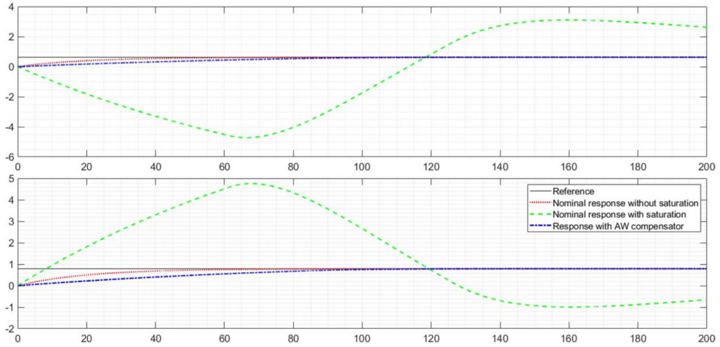
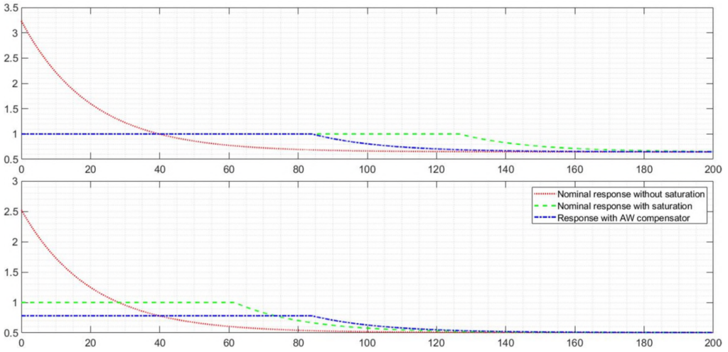
The system responses have been simulated for a step command at $t=0$ for the nominal system without saturation, with saturation and with saturation and anti-windup compensator in the following two figures respectively. As can be seen, the control performance hugely degrades in case the saturation nonlinearity is included. Moreover, when the anti-windup compensator is added to the control loop, performance can almost be recovered. Further details are found in [10].