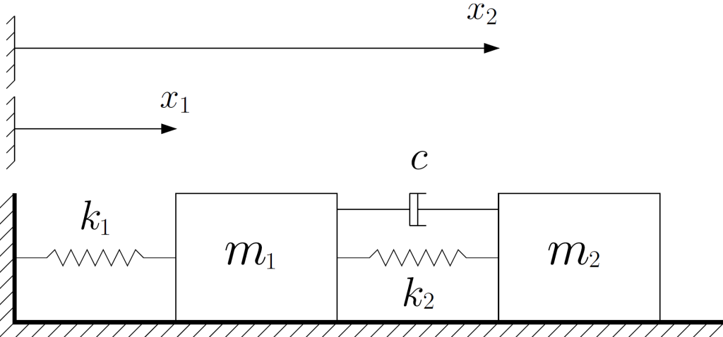
Robust estimator design for a mass-spring-damper system

The file Demo_014.m is found in IQClab’s folder demos; it performs a robust estimator synthesis with the function fRobest for a mass-spring-damper problem derived from the example presented in [24]. The setup is shown in the following figure.

The numerical values are $m_1=1$ , $m_2=0.5$ , $k_1=1$ , $k_2=1+0.5\delta_\mathrm{k}$ and $c=2+1.75\delta_\mathrm{c}$ with $\delta_\mathrm{k},\delta_\mathrm{c}\in[-1,1]$ . The first mass is disturbed by an external force $w_1$ . The objective is to estimate $x_2$ using a measument of $x_1$ corrupted by measurement noise $w_2$ . The linear fractional representation can then be written as

$\left(\!\!\begin{array}{c}q_\mathrm{c}\\q_\mathrm{k}\\z\\y\end{array}\!\!\right)= \left[\!\!\begin{array}{cccc|cccc}0&0&1&0&0&0&0&0\\ 0&0&0&1&0&0&0&0\\ -2&1&-2&2&-1.75&-0.5&1&0\\ 2&-2&4&-4&3.5&1&0&0\\ \hline 0&0&1&-1&0&0&0&0\\ 1&-1&0&0&0&0&0&0\\ 0&1&0&0&0&0&0&0\\ 1&0&0&0&0&0&0&1\end{array}\!\!\right] \left(\!\!\begin{array}{c}p_\mathrm{c}\\p_\mathrm{k}\\w_1\\w_2\end{array}\!\!\right)$

with $p_\mathrm{c}=\delta_\mathrm{c} q_\mathrm{c}$ , $p_\mathrm{k}=\delta_\mathrm{k} q_\mathrm{k}$ .

For comparison reasons, we design a nominal $H_2$ estimator, $E_\mathrm{nom}$ , using the function ‘h2syn’, which is part of MATLAB’s robust control toolbox, as well as a robust $H_2$ estimator, $E_\mathrm{rob}$ , using the function ‘fRobest’, which is part of IQClab.

The code for designing the nominal estimator is found in the file Demo_014.m. Designing the robust estimator proceeds as follows:

% Define plant (see script for system matrices) 
H = ss(A,[Bp,Bw],[Cq;Cz;Cy],[Dqp,Dqw;Dzp,Dzw;Dyp,Dyw]);

% Define uncertainties
de1 = iqcdelta('de1','InputChannel',1,'OutputChannel',1, 'Bounds',[-1,1]);
de1 = iqcassign(de1,'ultis','Length',3);

de2 = iqcdelta('de2','InputChannel',2,'OutputChannel',2, 'Bounds',[-1,1]);
de2 = iqcassign(de2,'ultis','Length',3);

% set options
options.perf      = 'H2';
options.StrProp   = 'yes';
options.subopt    = 1.03;
options.constants = 1e-8*ones(1,4);
options.Pi11pos   = 1e-8;
options.FeasbRad  = 1e9;

[Erob,gamrob]     = fRobest(H,{de1,de2},[2,1,1],[2,2],options);

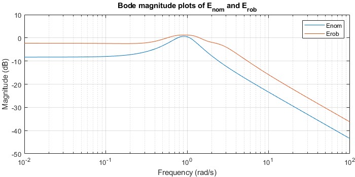
We obtain a nominal and robust estimator, $E_\mathrm{nom}$ and $E_\mathrm{rob}$ respectively, which guarantee a nominal and robust $H_2$ performance level of $0.82$ and $1.78$ respectively. The corresponding Bode-magnitude plots are depicted in the following figure.

Given $E_\mathrm{nom}$ and $E_\mathrm{rob}$ we can also perform a robustness analysis using the function ‘iqcanalysis’. This yields the following computed worst-case $H_2$ perfomormance levels for increasing levels of $\alpha$ with $|\delta_\mathrm{c}|<\alpha$ , $|\delta_\mathrm{k}|<\alpha$ .

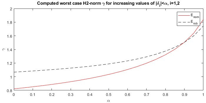
As can be seen, the nominal estimator, $E_\mathrm{nom}$ , shows better performance levels for smaller values of $\alpha$ , while for $\alpha>0.9$ the robust estimator, $E_\mathrm{rob}$ , outperforms $E_\mathrm{nom}$ .

To continue, let us also show some time-domain simulations, where we perturb the system with a random force disturbance and for different values of $\delta_\mathrm{k}=\delta_\mathrm{c}\in[-1,1]$ . The results are shown in the following two figures for $E_\mathrm{nom}$ and $E_\mathrm{rob}$ respectively.

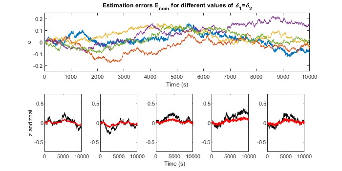
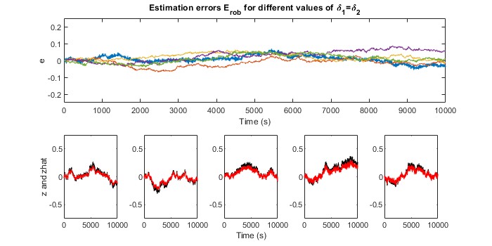
As can be seen, the robust estimator $E_\mathrm{rob}$ does a better job, if compared to $E_\mathrm{nom}$ . This is confirmed by the computed RMS values which are given in the following table.

\delta_\mathrm{k}=\delta_\mathrm{c}= — Computed RMS values for different values of the uncertainties.

$\delta_\mathrm{k}=\delta_\mathrm{c}=$	$-1$	$-0.5$	$0$	$0.5$	$1$	Mean
RMS value $E_\mathrm{nom}$	0.059	0.069	0.074	0.111	0.068	0.076
RMS value $E_\mathrm{rob}$	0.022	0.026	0.028	0.043	0.026	0.029