Anti-windup compensator design

IQClab also offers the possibility to perform an anti-windup compensator design. This allows to design compensators that prevent integrator windup in case of large control errors and limited actuator power.

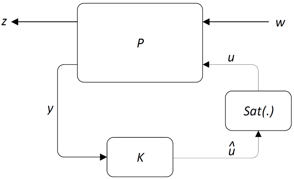
In case of saturation, we are coping with the configuration shown in the following figure, where $P$ is the generalized plant, $K$ the controller, and $\mathrm{sat}(\cdot)$ a standard saturation nonlinearity.

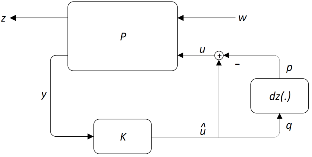
To pull out the saturation nonlinearity as an uncertainty, one can equivalently reformulate the interconnection as shown in the following figure with $\mathrm{sat}(\cdot)=1- \mathrm{dz} (\cdot)$ .

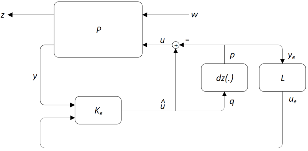
By now extending the controller $K=ss(A_K,B_K,C_K,D_K)$ as

$\hat{u}=\left[\!\begin{array}{c|ccc}A_K&B_K&I&0\\ \hline C_K&D_K&0&I\end{array}\!\right]\!\!\left(\!\!\!\begin{array}{c}y\\u_{e_1}\\u_{e_2}\end{array}\!\!\!\right),$

we can consider the interconnection shown in the following figure, where $u_e=Ly_e$ is the anti-windup compensator.

The corresponding generalized plant $P_e$ is therefore given by

$\left(\!\!\!\begin{array}{c}q\\z\\y_e\end{array}\!\!\!\right)\!=\!\left[\!\!\begin{array}{c|ccc}A&B_p&B_w&B_u\\ \hline C_q&D_{qp}&D_{qw}&D_{qu}\\C_\mathrm{z}&D_{zp}&D_{zw}&D_{zu}\\0&I&0&0\end{array}\!\!\right]\!\!\!\left(\!\!\begin{array}{c}p\\w\\u\end{array}\!\!\!\right),$

where

$p(\cdot)\in\mathbb{R}^{n_p}$ and $w(\cdot)\in\mathbb{R}^{n_w}$ are the uncertainty and disturbance inputs
$q(\cdot)\in\mathbb{R}^{n_q}$ and $z(\cdot)\in\mathbb{R}^{n_z}$ are the uncertainty and performance outputs
$u_e(\cdot)\in\mathbb{R}^{n_{u_e}}$ is the control input
$y_e(\cdot)\in\mathbb{R}^{n_{y_e}}$ is the measurement output

The design algorithm considered here is from [10]. This is an elementary, but potentially effective algorithm, which yields static compensators, while minimizing the induced $L_2$ -gain constraint on the performance channel $w\rightarrow z$ :

$\int_0^{\infty}\left(\begin{array}{c}z(t)\\w(t)\end{array}\right)^T\left(\begin{array}{cc}\frac{1}{\gamma}I&0\\0&-\gamma I\end{array}\right)\left(\begin{array}{c}z(t)\\w(t)\end{array}\right)dt\geq0\ \ \forall t\geq0.$

Here $\gamma$ is the to-be-minimized induced $L_2$ -gain.

Usage:

$[L,\gamma]=fAWsyn(P_e,n_{out},n_{in})$
$[L,\gamma]=fAWsyn(P_e,n_{out},n_{in},options)$

If feasible, the algorithms returns:

The anti-windup compensator gain $L$ .
The (guaranteed) induced $L_2$ -gain on the performance channel $w\rightarrow z$ of the closed-loop system $\Delta\star P_e\star L$ .

The inputs should be provided as follows:

The LTI plant $P_e$ is assumed to admit the state space description mentioned above.
The plant input and output dimension data $n_\mathrm{in}$ and $n_\mathrm{out}$ must be specified as follows:
- $n_\mathrm{in}=[n_p;n_w;n_u]$
- $n_\mathrm{out}=[n_q;n_z;n_y]$
The last input, options, is a structure with various options as summarized in the following table.

Options	Description
options.alpha	If specified, options.alpha defines the sector constraint $[0,\alpha]$ , $\alpha>0$ . The default value is 1.
options.constants	options.constants= $[c_1,c_2,c_3]$ is a vector of (small) nonnegative constants, which perturb the LMIs as $LMI_i\prec-c_i$ , $i\in\{1,2,3\}$ . The constants are associated with the following LMI constraints – $c_1$ perturbs the main solvability condition as $LMI_\mathrm{primal}\prec-c_1I$ – $c_2$ perturbs the Lyapunov matrix as $X\succ c_2I$ – $c_3$ perturbs the sector constraint IQC-multiplier matrix variable $M\succ c_3I$ . The default value is $[0,0,0]$ .
options.Parser	The option options.Parser specifies which parser is used: – options.Parser=’LMIlab’ – options.Parser=’Yalmip’ The default options is ‘LMIlab’.
options.Solver	The option options.Solver specifies which solver is used when considering Yalmip as parser. See https://yalmip.github.io/ for further info. The default solver is ‘mincx’.
options.FeasbRad	This option allows setting the feasibility radius of the optimization problem (see MATLAB → help → mincx for further details). The default value is 1e9.
options.Terminate	This option can be used to change the LMI solver options (see MATLAB → help → mincx for further details). The default value is 0.
options.RelAcc	This option can be used to change the LMI solver options (see MATLAB → help → mincx for further details). The default value is 1e-4.

Futher options

In addition to the previous algorithm, it is also possible to design dynamic robust or gain-scheduled anti-windup compensators using fRobsyn and fLPVsyn respectively.

The application of fRobsyn is clear. Here it is emphasized that this algorithm goes much beyond the previous approach (but is not convex):

fRobsyn yields dynamic compensators (rather than static ones with fAWsyn), potentially leading to better anti-windup performance.
fRobsyn allows to consider dynamic multipliers (i.e., Zames-Falb multipliers, which are included in the class usbsr). Again, this offers the potential for obtaining less conservative results.
fRobsyn allows to include additional uncertainties.

Regarding the application of fLPVsyn, this is illustrated in the following figure.

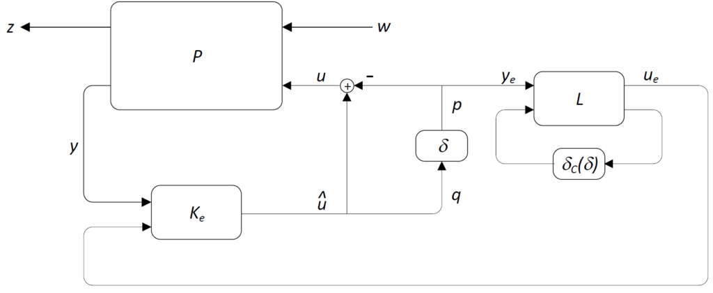
Here the deadzone nonlinearity was replaced by a time-varying parametric uncertainty $\delta=diag(\delta_1,\ldots,\delta_{n_u})$ . These are defined as $\delta_i(t)=1-\dfrac{u_i(t)}{\hat{u}_i(t)}$ .